subpixel | TheAILearner

In the previous blogs, we discussed how to find the corners using algorithms such as Harris Corner, Shi-Tomasi, etc. If you notice, the detected corners had integer coordinates such as (17,34), etc. This generally works if we were extracting these features for recognition purposes but when it comes to some geometrical measurements we need more precise corner locations such as real-valued coordinates (17.35,34.67). So, in this blog, we will see how to refine the corner locations (detected using Harris or Shi-Tomasi Detector) with sub-pixel accuracy.

OpenCV

OpenCV provides a builtin function cv2.cornerSubPix() that finds the sub-pixel accurate location of the corners. Below is the syntax of this

cv2.cornerSubPix(image, corners, winSize, zeroZone, criteria)

1	cv2.cornerSubPix(image, corners, winSize, zeroZone, criteria)

This function uses the dot product trick and iteratively refines the corner locations till the termination criteria is reaches. Let’s understand this in somewhat more detail.

Consider the image shown below. Suppose, q is the starting corner location and p is the point located within the neighborhood of q.

Clearly, the dot product between the gradient at p and the vector q-p is 0. For instance, for the first case because p₀ lies in a flat region, so the gradient is 0 and hence the dot product. For the second case, the vector q-p₁ lies on the edge and we know that the gradient is perpendicular to the edge so the dot product is 0.

Similarly, we take other points in the neighborhood of q (defined by the winSize parameter) and set the dot product of gradient at that point and the vector to 0 as we did above. Doing so we will get a system of equations. These equations form a linear system that can be solved by the inversion of a single autocorrelation matrix. But this matrix is not always invertible owing to small eigenvalues arising from the pixels very close to q. So, we simply reject the pixels in the immediate neighborhood of q (defined by the zeroZone parameter).

This will give us the new location for q. Now, this will become our starting corner location. Keep iterating until the user-specified termination criterion is reached. I hope you understood this.

Now, let’s take a look at the arguments that this function accepts.

image: Input single-channel, 8-bit grayscale or float image
corners: Array that holds the initial approximate location of corners
winSize: Size of the neighborhood where it searches for corners. This is the Half of the side length of the search window. For example, if winSize=Size(5,5) , then a (5∗2+1)×(5∗2+1)=11×11 search window is used
zeroZone: This is the half of the neighborhood size we want to reject. If you don’t want to reject anything pass (-1.-1)
criteria: Termination criteria. You can either stop it after a specified number of iterations or a certain accuracy is achieved, or whichever occurs first.

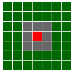
For instance, in the above image the red pixel is the initial corner. The winSize is (3,3) and the zeroZone is (1,1). So, only the green pixels have been considered for generating equations while the grey pixels have been rejected.

Now, let’s take the below image and see how to do this using OpenCV-Python

Steps

Load the image and find the corners using Harris Corner Detector as we did in the previous blog. You can use Shi-Tomasi detector also
Now, there may be a bunch of pixels at the corner, so we take their centroids
Then, we define the stopping criteria and refine the corners to subpixel accuracy using the cv2.cornerSubPix()
Finally, we used red color to mark Harris corners and green color to mark refined corners

import numpy as np
import cv2

# Load the image and convert to grayscale
img = cv2.imread('D:/downloads/contracing.png')
gray = cv2.cvtColor(img,cv2.COLOR_BGR2GRAY)

# find Harris corners as we did in the previous blog
gray = np.float32(gray)
dst = cv2.cornerHarris(gray,2,3,0.04)
dst = cv2.dilate(dst,None)
ret, dst = cv2.threshold(dst,0.01*dst.max(),255,0)
dst = np.uint8(dst)

# find centroids
ret, labels, stats, centroids = cv2.connectedComponentsWithStats(dst)

# define the criteria to stop. We stop it after a specified number of iterations
# or a certain accuracy is achieved, whichever occurs first.
criteria = (cv2.TERM_CRITERIA_EPS + cv2.TERM_CRITERIA_MAX_ITER, 100, 0.001)

# Refine the corners using cv2.cornerSubPix()
corners = cv2.cornerSubPix(gray,np.float32(centroids),(5,5),(-1,-1),criteria)

# To display, first convert the centroids and corners to integer
centroids = np.int0(centroids)
corners = np.int0(corners)

# then i have used red color to mark Harris Corners
# and green color to mark refined corners
img[centroids[:,1], centroids[:,0]]=[0,0,255]
img[corners[:,1], corners[:,0]] = [0,255,0]

# Write the image at the desired location
cv2.imwrite('D:/downloads/subpixel5.png',img)

import numpy as np

import cv2

# Load the image and convert to grayscale

img = cv2.imread('D:/downloads/contracing.png')

gray = cv2.cvtColor(img,cv2.COLOR_BGR2GRAY)

# find Harris corners as we did in the previous blog

gray = np.float32(gray)

dst = cv2.cornerHarris(gray,2,3,0.04)

dst = cv2.dilate(dst,None)

ret, dst = cv2.threshold(dst,0.01*dst.max(),255,0)

dst = np.uint8(dst)

# find centroids

ret, labels, stats, centroids = cv2.connectedComponentsWithStats(dst)

# define the criteria to stop. We stop it after a specified number of iterations

# or a certain accuracy is achieved, whichever occurs first.

criteria = (cv2.TERM_CRITERIA_EPS + cv2.TERM_CRITERIA_MAX_ITER, 100, 0.001)

# Refine the corners using cv2.cornerSubPix()

corners = cv2.cornerSubPix(gray,np.float32(centroids),(5,5),(-1,-1),criteria)

# To display, first convert the centroids and corners to integer

centroids = np.int0(centroids)

corners = np.int0(corners)

# then i have used red color to mark Harris Corners

# and green color to mark refined corners

img[centroids[:,1], centroids[:,0]]=[0,0,255]

img[corners[:,1], corners[:,0]] = [0,255,0]

# Write the image at the desired location

cv2.imwrite('D:/downloads/subpixel5.png',img)

Below are the results of this. For visualization, I have shown the zoomed in version on the right.

Applications

Subpixel corner locations are a common measurement used in camera calibration or when tracking to reconstruct the camera’s path or the three-dimensional structure of a tracked object or used in some algorithms such as SIFT (discussed in the next blog), etc.

That’s all for this blog. Hope you enjoy reading.

If you have any doubts/suggestions please feel free to ask and I will do my best to help or improve myself. Goodbye until next time.

Isn’t this an interesting topic? If you have worked with image classification problems( e.g. classifying cats and dogs) or image generation problems( e.g. GANs, autoencoders), surely you have encountered with convolution and deconvolution layer. But what if someone says a deconvolution layer is same as a convolution layer.

This paper has proposed an efficient subpixel convolution layer which works same as a deconvolution layer. To understand this, lets first understand convolution layer , transposed convolution layer and sub pixel convolution layer.

Convolution Layer

In every convolution neural network, convolution layer is the most important part. A convolution layer is consist of numbers of independent filters which convolve independently with input and produce output for the next layer. Let’s see how a filter convolve with the input.

Transposed and sub pixel Convolution Layer

Transposed convolution is the inverse operation of convolution. In convolution layer, you try to extract useful features from input while in transposed convolution, you try to add some useful features to upscale an image. Transposed convolution has learnable features which are learnt using backpropogation. Lets see how to do a transposed convolution visually.

Similarly, a subpixel convolution is also used for upsampling an image. It uses fractional strides( input is padded with in-between zero pixels) to an input and outputs an upsampled image. Let’s see visually.

An efficient sub pixel convolution Layer

In this paper authors have proposed that upsampling using deconvolution layer isn’t really necessary. So they came up with this Idea. Instead of putting in between zero pixels in the input image, they do more convolution in lower resolution image and then apply periodic shuffling to produce an upscaled image.

Authors have illustrated that deconvolution layer with kernel size of (o, i, k*r , k*r ) is same as convolution layer with kernel size of (o*r *r, i, k, k) e.g. (output channels, input channels, kernel width, kernel height) in LR space. Let’s take an example of proposed efficient subpixel convolution layer.

In the above figure, input image shape is (1, 4, 4) and upscaling ratio(r) is 2. To achieve an image of size (1, 8, 8), first input image is applied with kernel size of (4, 1, 2, 2) which produces output of shape (4, 4, 4) and then periodic shufling is applied to get required upscaled image of shape (1, 8, 8). So instead of using deconvolution layer with kernel size of (1, 1, 4, 4) same can be done with this efficient sub pixel convolution layer.

Implementation

I have also implemented an autoencoder(using MNIST dataset) with efficient subpixel convolution layer. Let’s see the code for efficient subpixel convolution.

def _phase_shift(I, r):  # defines periodical shuffling to upscale image
    input_shape = tf.shape(I)
    bsize = input_shape[0]
    a = input_shape[1]
    b = input_shape[2]
    c = tf.cast(input_shape[3]/(r ** 2),tf.int32)
    shape = tf.stack([bsize,a,b,r,r,c])

    input_shape_as_numbers = I.get_shape()

    X = tf.reshape(tensor=I, shape=shape)
    X = tf.transpose(X, (0, 1, 2, 4, 3,5))  
    X = tf.split(X, input_shape_as_numbers[1], axis=1)  
    X = tf.concat([tf.squeeze(x) for x in X], axis=2)  
    X = tf.split(X,input_shape_as_numbers[2], axis=1) 
    X = tf.concat([tf.squeeze(x) for x in X], axis=2) 

    return tf.reshape(X, (bsize, a*r, b*r, c))

def PS(input_shape, r, name, color=False):

    def subpixel_shape(input_shape):
        dims = [input_shape[0],
            input_shape[1] * r,
            input_shape[2] * r,
            int(input_shape[3] / (r ** 2))]
        output_shape = tuple(dims)
        return output_shape
  
    def subpixel(x):
        if color:
            Xc = tf.split(3, 3, X)
            X = tf.concat(3, [_phase_shift(x, r) for x in Xc])
        else:
            x_upsampled = _phase_shift(x, r)
        return x_upsampled

    return Lambda(subpixel, output_shape=subpixel_shape, name=name)


# encoder layers
encoder_inputs = Input(shape = (28,28,1))
conv1 = Conv2D(16, (3,3), activation = 'relu', padding = "SAME")(encoder_inputs)
pool1 = MaxPooling2D(pool_size = (2,2), strides = 2)(conv1)
conv2 = Conv2D(32, (3,3), activation = 'relu', padding = "SAME")(pool1)
pool2 = MaxPooling2D(pool_size = (2,2), strides = 2)(conv2)
flat = Flatten()(pool2)

#decoder layer
dense_layer_d = Dense(7*7*32, activation = 'relu')(enocder_outputs)
output_from_d = Reshape((7,7,32))(dense_layer_d)

# convolution then periodical shuffling to upscale image
sub_up = Conv2D(128, (2,2), activation = 'relu', padding = "SAME")(output_from_d)
upSampled_1 = PS(sub_up.shape, 2, name = 'subpixel1', color=False)(sub_up)

output_from_upSampled_1 = Reshape((14,14,32))(upSampled_1)

# convolution then periodical shuffling to upscale image
sub_up_2 = Conv2D(4, (2,2), activation = 'relu', padding = "SAME")(output_from_upSampled_1)
output = PS(sub_up_2.shape, 2, name = 'subpixel2', color=False)(sub_up_2)

autoencoder = Model(encoder_inputs, output)

# training of model
m = 256
n_epoch = 25
autoencoder.compile(optimizer='adam', loss='mse')
autoencoder.fit(output_X_train,output_X_train, epochs=n_epoch, batch_size=m, shuffle=True)

def _phase_shift(I, r): # defines periodical shuffling to upscale image

input_shape = tf.shape(I)

bsize = input_shape[0]

a = input_shape[1]

b = input_shape[2]

c = tf.cast(input_shape[3]/(r ** 2),tf.int32)

shape = tf.stack([bsize,a,b,r,r,c])

input_shape_as_numbers = I.get_shape()

X = tf.reshape(tensor=I, shape=shape)

X = tf.transpose(X, (0, 1, 2, 4, 3,5))

X = tf.split(X, input_shape_as_numbers[1], axis=1)

X = tf.concat([tf.squeeze(x) for x in X], axis=2)

X = tf.split(X,input_shape_as_numbers[2], axis=1)

X = tf.concat([tf.squeeze(x) for x in X], axis=2)

return tf.reshape(X, (bsize, a*r, b*r, c))

def PS(input_shape, r, name, color=False):

def subpixel_shape(input_shape):

dims = [input_shape[0],

input_shape[1] * r,

input_shape[2] * r,

int(input_shape[3] / (r ** 2))]

output_shape = tuple(dims)

return output_shape

def subpixel(x):

if color:

Xc = tf.split(3, 3, X)

X = tf.concat(3, [_phase_shift(x, r) for x in Xc])

else:

x_upsampled = _phase_shift(x, r)

return x_upsampled

return Lambda(subpixel, output_shape=subpixel_shape, name=name)

# encoder layers

encoder_inputs = Input(shape = (28,28,1))

conv1 = Conv2D(16, (3,3), activation = 'relu', padding = "SAME")(encoder_inputs)

pool1 = MaxPooling2D(pool_size = (2,2), strides = 2)(conv1)

conv2 = Conv2D(32, (3,3), activation = 'relu', padding = "SAME")(pool1)

pool2 = MaxPooling2D(pool_size = (2,2), strides = 2)(conv2)

flat = Flatten()(pool2)

#decoder layer

dense_layer_d = Dense(7*7*32, activation = 'relu')(enocder_outputs)

output_from_d = Reshape((7,7,32))(dense_layer_d)

# convolution then periodical shuffling to upscale image

sub_up = Conv2D(128, (2,2), activation = 'relu', padding = "SAME")(output_from_d)

upSampled_1 = PS(sub_up.shape, 2, name = 'subpixel1', color=False)(sub_up)

output_from_upSampled_1 = Reshape((14,14,32))(upSampled_1)

# convolution then periodical shuffling to upscale image

sub_up_2 = Conv2D(4, (2,2), activation = 'relu', padding = "SAME")(output_from_upSampled_1)

output = PS(sub_up_2.shape, 2, name = 'subpixel2', color=False)(sub_up_2)

autoencoder = Model(encoder_inputs, output)

# training of model

m = 256

n_epoch = 25

autoencoder.compile(optimizer='adam', loss='mse')

autoencoder.fit(output_X_train,output_X_train, epochs=n_epoch, batch_size=m, shuffle=True)

The above periodic shuffling code is given by this github link. Then applied autoencoder layers to generate image. To up-sample image in decoder layers first convolved encoded images then used periodical shuffling.

This type of subpixel convolution layers can be very helpful in problems like image generation( autoencoders, GANs), image enhancement(super resolution). Also there is more to find out what can this efficient subpixel convolution layer offers.

Now, you might have got some feeling about efficient subpixel convolution layer. Hope you enjoy reading.

If you have any doubt/suggestion please feel free to ask and I will do my best to help or improve myself. Good-bye until next time.

Referenced Research Paper : Is the deconvolution layer the same as a convolutional layer?

Referenced Gitub Link : Subpixel

TheAILearner

Mastering Artificial Intelligence

Tag Archives: subpixel

Finding Corners with SubPixel Accuracy

OpenCV

Steps

Applications

Is the deconvolution layer the same as a convolutional layer?