Tag Archives: python

Is the deconvolution layer the same as a convolutional layer?

Isn’t this an interesting topic? If you have worked with image classification problems( e.g. classifying cats and dogs) or image generation problems( e.g. GANs, autoencoders), surely you have encountered with convolution and deconvolution layer. But what if someone says a deconvolution layer is same as a convolution layer.

This paper has proposed an efficient subpixel convolution layer which works same as a deconvolution layer. To understand this, lets first understand convolution layer , transposed convolution layer and sub pixel convolution layer.

Convolution Layer

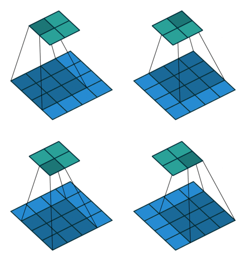
In every convolution neural network, convolution layer is the most important part. A convolution layer is consist of numbers of independent filters which convolve independently with input and produce output for the next layer. Let’s see how a filter convolve with the input.

Transposed and sub pixel Convolution Layer

Transposed convolution is the inverse operation of convolution. In convolution layer, you try to extract useful features from input while in transposed convolution, you try to add some useful features to upscale an image. Transposed convolution has learnable features which are learnt using backpropogation. Lets see how to do a transposed convolution visually.

Similarly, a subpixel convolution is also used for upsampling an image. It uses fractional strides( input is padded with in-between zero pixels) to an input and outputs an upsampled image. Let’s see visually.

An efficient sub pixel convolution Layer

In this paper authors have proposed that upsampling using deconvolution layer isn’t really necessary. So they came up with this Idea. Instead of putting in between zero pixels in the input image, they do more convolution in lower resolution image and then apply periodic shuffling to produce an upscaled image.

Authors have illustrated that deconvolution layer with kernel size of (o, i, k*r , k*r ) is same as convolution layer with kernel size of (o*r *r, i, k, k) e.g. (output channels, input channels, kernel width, kernel height) in LR space. Let’s take an example of proposed efficient subpixel convolution layer.

In the above figure, input image shape is (1, 4, 4) and upscaling ratio(r) is 2. To achieve an image of size (1, 8, 8), first input image is applied with kernel size of (4, 1, 2, 2) which produces output of shape (4, 4, 4) and then periodic shufling is applied to get required upscaled image of shape (1, 8, 8). So instead of using deconvolution layer with kernel size of (1, 1, 4, 4) same can be done with this efficient sub pixel convolution layer.

Implementation

I have also implemented an autoencoder(using MNIST dataset) with efficient subpixel convolution layer. Let’s see the code for efficient subpixel convolution.

def _phase_shift(I, r):  # defines periodical shuffling to upscale image
    input_shape = tf.shape(I)
    bsize = input_shape[0]
    a = input_shape[1]
    b = input_shape[2]
    c = tf.cast(input_shape[3]/(r ** 2),tf.int32)
    shape = tf.stack([bsize,a,b,r,r,c])

    input_shape_as_numbers = I.get_shape()

    X = tf.reshape(tensor=I, shape=shape)
    X = tf.transpose(X, (0, 1, 2, 4, 3,5))  
    X = tf.split(X, input_shape_as_numbers[1], axis=1)  
    X = tf.concat([tf.squeeze(x) for x in X], axis=2)  
    X = tf.split(X,input_shape_as_numbers[2], axis=1) 
    X = tf.concat([tf.squeeze(x) for x in X], axis=2) 

    return tf.reshape(X, (bsize, a*r, b*r, c))

def PS(input_shape, r, name, color=False):

    def subpixel_shape(input_shape):
        dims = [input_shape[0],
            input_shape[1] * r,
            input_shape[2] * r,
            int(input_shape[3] / (r ** 2))]
        output_shape = tuple(dims)
        return output_shape
  
    def subpixel(x):
        if color:
            Xc = tf.split(3, 3, X)
            X = tf.concat(3, [_phase_shift(x, r) for x in Xc])
        else:
            x_upsampled = _phase_shift(x, r)
        return x_upsampled

    return Lambda(subpixel, output_shape=subpixel_shape, name=name)


# encoder layers
encoder_inputs = Input(shape = (28,28,1))
conv1 = Conv2D(16, (3,3), activation = 'relu', padding = "SAME")(encoder_inputs)
pool1 = MaxPooling2D(pool_size = (2,2), strides = 2)(conv1)
conv2 = Conv2D(32, (3,3), activation = 'relu', padding = "SAME")(pool1)
pool2 = MaxPooling2D(pool_size = (2,2), strides = 2)(conv2)
flat = Flatten()(pool2)

#decoder layer
dense_layer_d = Dense(7*7*32, activation = 'relu')(enocder_outputs)
output_from_d = Reshape((7,7,32))(dense_layer_d)

# convolution then periodical shuffling to upscale image
sub_up = Conv2D(128, (2,2), activation = 'relu', padding = "SAME")(output_from_d)
upSampled_1 = PS(sub_up.shape, 2, name = 'subpixel1', color=False)(sub_up)

output_from_upSampled_1 = Reshape((14,14,32))(upSampled_1)

# convolution then periodical shuffling to upscale image
sub_up_2 = Conv2D(4, (2,2), activation = 'relu', padding = "SAME")(output_from_upSampled_1)
output = PS(sub_up_2.shape, 2, name = 'subpixel2', color=False)(sub_up_2)

autoencoder = Model(encoder_inputs, output)

# training of model
m = 256
n_epoch = 25
autoencoder.compile(optimizer='adam', loss='mse')
autoencoder.fit(output_X_train,output_X_train, epochs=n_epoch, batch_size=m, shuffle=True)

def _phase_shift(I, r): # defines periodical shuffling to upscale image

input_shape = tf.shape(I)

bsize = input_shape[0]

a = input_shape[1]

b = input_shape[2]

c = tf.cast(input_shape[3]/(r ** 2),tf.int32)

shape = tf.stack([bsize,a,b,r,r,c])

input_shape_as_numbers = I.get_shape()

X = tf.reshape(tensor=I, shape=shape)

X = tf.transpose(X, (0, 1, 2, 4, 3,5))

X = tf.split(X, input_shape_as_numbers[1], axis=1)

X = tf.concat([tf.squeeze(x) for x in X], axis=2)

X = tf.split(X,input_shape_as_numbers[2], axis=1)

X = tf.concat([tf.squeeze(x) for x in X], axis=2)

return tf.reshape(X, (bsize, a*r, b*r, c))

def PS(input_shape, r, name, color=False):

def subpixel_shape(input_shape):

dims = [input_shape[0],

input_shape[1] * r,

input_shape[2] * r,

int(input_shape[3] / (r ** 2))]

output_shape = tuple(dims)

return output_shape

def subpixel(x):

if color:

Xc = tf.split(3, 3, X)

X = tf.concat(3, [_phase_shift(x, r) for x in Xc])

else:

x_upsampled = _phase_shift(x, r)

return x_upsampled

return Lambda(subpixel, output_shape=subpixel_shape, name=name)

# encoder layers

encoder_inputs = Input(shape = (28,28,1))

conv1 = Conv2D(16, (3,3), activation = 'relu', padding = "SAME")(encoder_inputs)

pool1 = MaxPooling2D(pool_size = (2,2), strides = 2)(conv1)

conv2 = Conv2D(32, (3,3), activation = 'relu', padding = "SAME")(pool1)

pool2 = MaxPooling2D(pool_size = (2,2), strides = 2)(conv2)

flat = Flatten()(pool2)

#decoder layer

dense_layer_d = Dense(7*7*32, activation = 'relu')(enocder_outputs)

output_from_d = Reshape((7,7,32))(dense_layer_d)

# convolution then periodical shuffling to upscale image

sub_up = Conv2D(128, (2,2), activation = 'relu', padding = "SAME")(output_from_d)

upSampled_1 = PS(sub_up.shape, 2, name = 'subpixel1', color=False)(sub_up)

output_from_upSampled_1 = Reshape((14,14,32))(upSampled_1)

# convolution then periodical shuffling to upscale image

sub_up_2 = Conv2D(4, (2,2), activation = 'relu', padding = "SAME")(output_from_upSampled_1)

output = PS(sub_up_2.shape, 2, name = 'subpixel2', color=False)(sub_up_2)

autoencoder = Model(encoder_inputs, output)

# training of model

m = 256

n_epoch = 25

autoencoder.compile(optimizer='adam', loss='mse')

autoencoder.fit(output_X_train,output_X_train, epochs=n_epoch, batch_size=m, shuffle=True)

The above periodic shuffling code is given by this github link. Then applied autoencoder layers to generate image. To up-sample image in decoder layers first convolved encoded images then used periodical shuffling.

This type of subpixel convolution layers can be very helpful in problems like image generation( autoencoders, GANs), image enhancement(super resolution). Also there is more to find out what can this efficient subpixel convolution layer offers.

Now, you might have got some feeling about efficient subpixel convolution layer. Hope you enjoy reading.

If you have any doubt/suggestion please feel free to ask and I will do my best to help or improve myself. Good-bye until next time.

Referenced Research Paper : Is the deconvolution layer the same as a convolutional layer?

Referenced Gitub Link : Subpixel

Python Closures

Leave a reply

Python Closures are related to nested functions(a function defined inside another function). As we have discussed in the previous blog, nested functions can access the variables from the enclosing scope that can be modified using the nonlocal keyword.

You cannot call these variables outside their scopes but closure remembers these values even if they are not present in the memory.

Now, let’s see how to define a closure

def name(text):          # outer enclosing function

    def print_name():    # nested function

        print(text)

    return print_name

name_closure = name("Pankaj")
name_closure()

def name(text): # outer enclosing function

def print_name(): # nested function

print(text)

return print_name

name_closure = name("Pankaj")

name_closure()

Here, the enclosing function returns the nested function instead of calling it. This returned function was bound to name_closure. On calling name_closure(), the name was still remembered although we had already finished executing the enclosing function.

This can be used for data hiding and a substitute for classes if we have only one method in the class (Always prefer using class over this according to me).

You can check for closure function with the help of __closure__ attribute. This returns a tuple of cell objects if it is a closure function otherwise prints nothing as shown below

>>> name_closure.__closure__
(<cell at 0x0000001F8D4FC528: str object at 0x0000001F8D51FEA0>,)
>>> name.__closure__
>>>

>>> name_closure.__closure__

(<cell at 0x0000001F8D4FC528: str object at 0x0000001F8D51FEA0>,)

>>> name.__closure__

>>>

In the next blog, we will learn decorators that use closures as well. Hope you enjoy reading.

If you have any doubt/suggestion please feel free to ask and I will do my best to help or improve myself. Good-bye until next time.

Densely Connected Convolutional Networks – DenseNet

1 Reply

When we see a machine learning problem related to an image, the first things comes into our mind is CNN(convolutional neural networks). Different convolutional networks like LeNet, AlexNet, VGG16, VGG19, ResNet, etc. are used to solve different problems either it is supervised(classification) or unsupervised(image generation). Through these years there has been more deeper and deeper CNN architectures are used. As more complex problem comes, more deeper convolutional networks are preferred. But with deeper networks problem of vanishing gradient arises.

To solve this problem Gao Huang et al. introduced Dense Convolutional networks. DenseNets have several compelling advantages:

alleviate the vanishing-gradient problem
strengthen feature propagation
encourage feature reuse, and substantially reduce the number of parameters.

How DenseNet works?

Recent researches like ResNet also tries to solve the problem of vanishing gradient. ResNet passes information from one layer to another layer via identity connection. In ResNet features are combined through summation before passing into the next layer.

While in DenseNet, it introduces connection from one layer to all its subsequent layer in a feed forward fashion (As shown in the figure below). This connection is done using concatenation not through summation.

source: DenseNet

ResNet architecture preserve information explicitly through identity connection, also recent variation of ResNet shows that many layers contribute very little and can in fact be randomly dropped during training. DenseNet architecture explicitly differentiates between information that is added to the network and information that is preserved.

In DenseNet, Each layer has direct access to the gradients from the loss function and the original input signal, leading to an r improved flow of information and gradients throughout the network, DenseNets have a regularizing effect, which reduces overfitting on tasks with smaller training set sizes.

An important difference between DenseNet and existing network architectures is that DenseNet can have very narrow layers, e.g., k = 12. It refers to the hyperparameter k as the growth rate of the network. It means each layer in dense block will only produce k features. And these k features will be concatenated with previous layers features and will be given as input to the next layer.

DenseNet Architecture

The best way to illustrate any architecture is done with the help of code. So, I have implemented DenseNet architecture in Keras using MNIST data set.

A DenseNet consists of dense blocks. Each dense block consists of convolution layers. After a dense block a transition layer is added to proceed to next dense block (As shown in figure below).

Every layer in a dense block is directly connected to all its subsequent layers. Consequently, each layer receives the feature-maps of all preceding layer.

def dense_block(block_x, filters, growth_rate):
    for i in range(layers_in_block):
        each_layer = conv_layer(block_x, growth_rate)
        block_x = concatenate([block_x, each_layer], axis=-1)
        filters += growth_rate

    return block_x, filters

def dense_block(block_x, filters, growth_rate):

for i in range(layers_in_block):

each_layer = conv_layer(block_x, growth_rate)

block_x = concatenate([block_x, each_layer], axis=-1)

filters += growth_rate

return block_x, filters

Each convolution layer is consist of three consecutive operations: batch normalization (BN) , followed by a rectified linear unit (ReLU) and a 3 × 3 convolution (Conv). Also dropout can be added which depends on your architecture requirement.

def conv_layer(conv_x, filters): 
    conv_x = BatchNormalization()(conv_x)
    conv_x = Activation('relu')(conv_x)
    conv_x = Conv2D(filters, (3, 3), kernel_initializer='he_uniform', padding='same', use_bias=False)(conv_x)
    conv_x = Dropout(0.2)(conv_x)

    return conv_x

def conv_layer(conv_x, filters):

conv_x = BatchNormalization()(conv_x)

conv_x = Activation('relu')(conv_x)

conv_x = Conv2D(filters, (3, 3), kernel_initializer='he_uniform', padding='same', use_bias=False)(conv_x)

conv_x = Dropout(0.2)(conv_x)

return conv_x

An essential part of convolutional networks is down-sampling layers that change the size of feature-maps. To facilitate down-sampling in DenseNet architecture it divides the network into multiple densely connected dense blocks(As shown in figure earlier).

The layers between blocks are transition layers, which do convolution and pooling. The transition layers consist of a batch normalization layer and an 1×1 convolutional layer followed by a 2×2 average pooling layer.

def transition_block(trans_x, tran_filters):
    trans_x = BatchNormalization()(trans_x)
    trans_x = Activation('relu')(trans_x)
    trans_x = Conv2D(tran_filters, (1, 1), kernel_initializer='he_uniform', padding='same', use_bias=False)(trans_x)
    trans_x = AveragePooling2D((2, 2), strides=(2, 2))(trans_x)

    return trans_x, tran_filters

def transition_block(trans_x, tran_filters):

trans_x = BatchNormalization()(trans_x)

trans_x = Activation('relu')(trans_x)

trans_x = Conv2D(tran_filters, (1, 1), kernel_initializer='he_uniform', padding='same', use_bias=False)(trans_x)

trans_x = AveragePooling2D((2, 2), strides=(2, 2))(trans_x)

return trans_x, tran_filters

DenseNets can scale naturally to hundreds of layers, while exhibiting no optimization difficulties. Because of their compact internal representations and reduced feature redundancy, DenseNets may be good feature extractors for various computer vision tasks that build on convolutional features

The full code can be found here.

Referenced research paper: Densely Connected Convolutional Networks

Hope you enjoy reading. If you have any doubt/suggestion please feel free to ask and I will do my best to help or improve myself. Good-bye until next time.

Object Tracking Using Color Models OpenCV-Python

Leave a reply

In this tutorial, we will learn how we can use color models for object tracking. You can use any color model. Here, I have used HSI because it is easier to represent a color using the HSI model (as it separates the color component from greyscale). Let’s see how to do this

Steps

Open the camera using cv2.VideoCapture()
Create 3 Trackbars of H, S, and I using cv2.createTrackbar()
Read frame by frame
Record the current trackbar position using cv2.getTrackbarPos()
Convert from BGR to HSV using cv2.cvtColor()
Threshold the HSV image based on current trackbar position using cv2.inRange()
Extract the desired result

Code

import cv2
import numpy as np

def nothing(x):
    pass

cap = cv2.VideoCapture(0) 

# Create a window
cv2.namedWindow('image',cv2.WINDOW_NORMAL)


# create trackbars for color change
cv2.createTrackbar('lowH','image',0,179,nothing)
cv2.createTrackbar('highH','image',179,179,nothing)

cv2.createTrackbar('lowS','image',0,255,nothing)
cv2.createTrackbar('highS','image',255,255,nothing)

cv2.createTrackbar('lowV','image',0,255,nothing)
cv2.createTrackbar('highV','image',255,255,nothing)

while(True):
    ret, frame = cap.read()

    # get current positions of the trackbars
    ilowH = cv2.getTrackbarPos('lowH', 'image')
    ihighH = cv2.getTrackbarPos('highH', 'image')
    ilowS = cv2.getTrackbarPos('lowS', 'image')
    ihighS = cv2.getTrackbarPos('highS', 'image')
    ilowV = cv2.getTrackbarPos('lowV', 'image')
    ihighV = cv2.getTrackbarPos('highV', 'image')

    hsv = cv2.cvtColor(frame, cv2.COLOR_BGR2HSV)
    lower_hsv = np.array([ilowH, ilowS, ilowV])
    higher_hsv = np.array([ihighH, ihighS, ihighV])
    mask = cv2.inRange(hsv, lower_hsv, higher_hsv)

    frame = cv2.bitwise_and(frame, frame, mask=mask)
    cv2.imshow('image', frame)
    if cv2.waitKey(1) & 0xFF == ord('q'):
        break

cap.release()
cv2.destroyAllWindows()

import cv2

import numpy as np

def nothing(x):

pass

cap = cv2.VideoCapture(0)

# Create a window

cv2.namedWindow('image',cv2.WINDOW_NORMAL)

# create trackbars for color change

cv2.createTrackbar('lowH','image',0,179,nothing)

cv2.createTrackbar('highH','image',179,179,nothing)

cv2.createTrackbar('lowS','image',0,255,nothing)

cv2.createTrackbar('highS','image',255,255,nothing)

cv2.createTrackbar('lowV','image',0,255,nothing)

cv2.createTrackbar('highV','image',255,255,nothing)

while(True):

ret, frame = cap.read()

# get current positions of the trackbars

ilowH = cv2.getTrackbarPos('lowH', 'image')

ihighH = cv2.getTrackbarPos('highH', 'image')

ilowS = cv2.getTrackbarPos('lowS', 'image')

ihighS = cv2.getTrackbarPos('highS', 'image')

ilowV = cv2.getTrackbarPos('lowV', 'image')

ihighV = cv2.getTrackbarPos('highV', 'image')

hsv = cv2.cvtColor(frame, cv2.COLOR_BGR2HSV)

lower_hsv = np.array([ilowH, ilowS, ilowV])

higher_hsv = np.array([ihighH, ihighS, ihighV])

mask = cv2.inRange(hsv, lower_hsv, higher_hsv)

frame = cv2.bitwise_and(frame, frame, mask=mask)

cv2.imshow('image', frame)

if cv2.waitKey(1) & 0xFF == ord('q'):

break

cap.release()

cv2.destroyAllWindows()

Open in full screen and play with trackbar to get more intuition about HSI model. Hope you enjoy reading.

If you have any doubt/suggestion please feel free to ask and I will do my best to help or improve myself. Good-bye until next time.

Color Models

Leave a reply

In the previous blogs, we represented the color image using the RGB components but this is not the only way available. There are different color models ( A color model is simply a way to define the color) available, each having their own pros and cons.

There are two types of color models available: Additive and Subtractive. Additive uses light (transmitted) to display color while subtractive models use printing inks. These models are fitted into different shapes to obtain new models (See HSI model below).

In this blog, we’ll discuss the three that are most commonly used in the context of digital image processing: RGB, CMY, and HSI

The RGB Color Model

In this, we construct a color cube whose 3 axes denote R, G, and B respectively as shown below

Normalized RGB Color Cube; Source: Researchgate

This is an additive model, i.e. the colors present in the light add to form new colors. For example, Yellow has coordinate of (1,1,0) which means Yellow = Red + Green. Similarly, for other colors like cyan = Blue + Green and magenta = Red +Blue.

R, G, and B are added together in varying proportions to produce an extensive range of colors. Mixing equal proportions of R, G, and B falls on the grayscale line.

Use: color monitors and most video cameras.

The CMYK Color Model

CMY stands for cyan, magenta, and yellow also known as secondary colors of light. K refers to black. An equal proportion of C, M, and Y produce muddly black and not pure black. That’s why we use CMYK instead of CMY model.

This is a subtractive model i.e colors are perceived as a result of reflected light. e.g. when light falls on a cyan coated surface, red is absorbed (or subtracted) while Green and Blue are reflected and thus G + B = Cyan. Similarly for magenta and yellow.

Thus, CMY can be obtained from RGB by subtracting RGB from the max intensity.

Use: Printing like books, magazines etc.

The HSI Color Model

HSI stands for Hue, Saturation, and Intensity. This model is similar to how humans perceive color. Let’s understand HSI terms

Hue: Color attribute that describes the pure color or dominant wavelength.

Saturation: Purity of Color or how much a pure color is diluted by white light.

Intensity: Amount of light

H and S tell us about the chromaticity (color information) of the light while I carries the greyscale information.

HSI model can be obtained by rotating the RGB cube such that Black is at the bottom and white at the top.

H varies from 0 to 120 degrees for Red, 120 – 240 for Green, and 240 -360 for Blue. Saturation can take value from 0 to 100%. Intensity value varies according to the bit size of an image.

Pros: Easier to represent the color than the RGB model.

Note: We can also use these color models for object tracking (See here).

In the next blog, we will see how different colors can be generated from these color models with the help of OpenCV. Hope you enjoy reading.

If you have any doubt/suggestion please feel free to ask and I will do my best to help or improve myself. Good-bye until next time.

Changing Video Resolution using OpenCV-Python

3 Replies

In this tutorial, I will show how to change the resolution of the video using OpenCV-Python. This blog is based on interpolation methods (Chapter-5) which we have discussed earlier.

Here, I will convert a 640×480 video to 1280×720. Let’s see how to do this

Steps:

Load a video using cv2.VideoCapture()
Create a VideoWriter object using cv2.VideoWriter()
Extract frame by frame
Resize the frames using cv2.resize()
Save the frames to a video file using cv2.VideoWriter()
Release the VideoWriter and destroy all windows

Code:

import cv2
import numpy as np

cap = cv2.VideoCapture('C:/New folder/video.avi')

fourcc = cv2.VideoWriter_fourcc(*'XVID')
out = cv2.VideoWriter('output.avi',fourcc, 5, (1280,720))

while True:
    ret, frame = cap.read()
    if ret == True:
        b = cv2.resize(frame,(1280,720),fx=0,fy=0, interpolation = cv2.INTER_CUBIC)
        out.write(b)
    else:
        break
    
cap.release()
out.release()
cv2.destroyAllWindows()

import cv2

import numpy as np

cap = cv2.VideoCapture('C:/New folder/video.avi')

fourcc = cv2.VideoWriter_fourcc(*'XVID')

out = cv2.VideoWriter('output.avi',fourcc, 5, (1280,720))

while True:

ret, frame = cap.read()

if ret == True:

b = cv2.resize(frame,(1280,720),fx=0,fy=0, interpolation = cv2.INTER_CUBIC)

out.write(b)

else:

break

cap.release()

out.release()

cv2.destroyAllWindows()

Here, I have used Bicubic as the interpolation method, you can use any. Hope you enjoy reading.

If you have any doubt/suggestion please feel free to ask and I will do my best to help or improve myself. Good-bye until next time.

Variational Autoencoders

Leave a reply

Variational autoencoders are an extension of autoencoders and used as generative models. You can generate data like text, images and even music with the help of variational autoencoders.

Autoencoders are the neural network used to reconstruct original input. To know more about autoencoders please got through this blog. They have a certain application like denoising autoencoders and dimensionality reduction for data visualization. But apart from that, they are fairly limited.

To overcome this limitation, variational autoencoders comes into place. A common autoencoder learns a function which does not train autoencoder to generate images from a particular distribution. Also, if you try to create a generative model using autoencoders, you do not want to generate data as therein input. You want the output data with some variations which mostly look like input data.

Variational Autoencoder Model

A variational autoencoder has encoder and decoder part mostly same as autoencoders, the difference is instead of creating a compact distribution from its encoder, it learns a latent variable model. These latent variables are used to create a probability distribution from which input for the decoder is generated. Another is, instead of using mean squared or cross entropy loss function (as in autoencoders ) it has its own loss function.

I will not go further into the mathematics behind it, Lets jump into the code which will give more understanding about variational autoencoders. To know more about the mathematics behind it please go through this tutorial.

I have implemented variational autoencoder in keras using MNIST dataset. So lets first download the data.

# download training and test data from mnist and reshape it

from keras.datasets import mnist
(X_train, Y_train), (X_test, Y_test) = mnist.load_data()
X_train = X_train.astype('float32') / 255.
X_train = X_train.reshape(-1,28,28,1)

X_test = X_test.astype('float32') / 255.
X_test = X_test.reshape(-1,28,28,1)
print(X_train.shape, X_test.shape)

# download training and test data from mnist and reshape it

from keras.datasets import mnist

(X_train, Y_train), (X_test, Y_test) = mnist.load_data()

X_train = X_train.astype('float32') / 255.

X_train = X_train.reshape(-1,28,28,1)

X_test = X_test.astype('float32') / 255.

X_test = X_test.reshape(-1,28,28,1)

print(X_train.shape, X_test.shape)

Now create an encoder model as it is created in autoencoders.

# Create encoder network

inputs = Input(shape = (28,28,1))
conv1 = Conv2D(16, (3,3), activation = 'relu', padding = "SAME")(inputs)
conv1_1 = Conv2D(16, (3,3), activation = 'relu', padding = "SAME")(conv1)
pool1 = MaxPooling2D(pool_size = (2,2), strides = 2)(conv1_1)
conv2 = Conv2D(32, (3,3), activation = 'relu', padding = "SAME")(pool1)
pool2 = MaxPooling2D(pool_size = (2,2), strides = 2)(conv2)

flat = Flatten()(pool2)
input_to_z = Dense(32, activation = 'relu')(flat)

# Create encoder network

inputs = Input(shape = (28,28,1))

conv1 = Conv2D(16, (3,3), activation = 'relu', padding = "SAME")(inputs)

conv1_1 = Conv2D(16, (3,3), activation = 'relu', padding = "SAME")(conv1)

pool1 = MaxPooling2D(pool_size = (2,2), strides = 2)(conv1_1)

conv2 = Conv2D(32, (3,3), activation = 'relu', padding = "SAME")(pool1)

pool2 = MaxPooling2D(pool_size = (2,2), strides = 2)(conv2)

flat = Flatten()(pool2)

input_to_z = Dense(32, activation = 'relu')(flat)

Latent Distribution Parameters and Function

Now encode the output of the encoder to latent distribution parameters. Here, I have created two parameters mu and sigma which represents the mean and standard distribution of the distribution.

latent_dim = 2 # dimension of latent variable
mu = Dense(latent_dim, name='mu')(input_to_z)
sigma = Dense(latent_dim, name='log_var')(input_to_z)

encoder = Model(inputs, mu)

latent_dim = 2 # dimension of latent variable

mu = Dense(latent_dim, name='mu')(input_to_z)

sigma = Dense(latent_dim, name='log_var')(input_to_z)

encoder = Model(inputs, mu)

Here I have taken latent space dimension equal to 2. This is the bottleneck which means we are passing our entire set of data to two single variables. So if we increase our latent space dimension to 5, 10 or higher, we can get better results in the output. But this will create more data in the bottleneck.

Now create a Gaussian distribution function with mean zero and standard deviation of 1. This distribution will give variation in the input to the decoder, which will help to get variation in the output. Then decoder will predict the output using distribution.

# create latent distribution function and generate vectors

def sampling(args):
    mu, sigma = args
    epsilon = K.random_normal(shape=(K.shape(mu)[0], latent_dim),
                              mean=0., stddev=1.)
    return mu + K.exp(sigma) * epsilon

z = Lambda(sampling)([mu, sigma])

#create decoder network which is reverse of encoder

decoder_inputs = Input(K.int_shape(z)[1:])
dense_layer_d = Dense(7*7*32, activation = 'relu')(decoder_inputs)
output_from_z_d = Reshape((7,7,32))(dense_layer_d)
trans1_d = Conv2DTranspose(32, 3, padding='same', activation='relu', strides=(2, 2))(output_from_z_d)
trans1_1_d = Conv2DTranspose(16, 3, padding='same', activation='relu', strides=(2, 2))(trans1_d)
trans2_d = Conv2DTranspose(1, 3, padding='same', activation='relu')(trans1_1_d)


decoder = Model(decoder_inputs, trans2_d)
z_decoded = decoder(z)

# create latent distribution function and generate vectors

def sampling(args):

mu, sigma = args

epsilon = K.random_normal(shape=(K.shape(mu)[0], latent_dim),

mean=0., stddev=1.)

return mu + K.exp(sigma) * epsilon

z = Lambda(sampling)([mu, sigma])

#create decoder network which is reverse of encoder

decoder_inputs = Input(K.int_shape(z)[1:])

dense_layer_d = Dense(7*7*32, activation = 'relu')(decoder_inputs)

output_from_z_d = Reshape((7,7,32))(dense_layer_d)

trans1_d = Conv2DTranspose(32, 3, padding='same', activation='relu', strides=(2, 2))(output_from_z_d)

trans1_1_d = Conv2DTranspose(16, 3, padding='same', activation='relu', strides=(2, 2))(trans1_d)

trans2_d = Conv2DTranspose(1, 3, padding='same', activation='relu')(trans1_1_d)

decoder = Model(decoder_inputs, trans2_d)

z_decoded = decoder(z)

Loss Function

For the loss function, a variational autoencoder uses the sum of two losses, one is the generative loss which is a binary cross entropy loss and measures how accurately the image is predicted, another is the latent loss, which is KL divergence loss, measures how closely a latent variable match Gaussian distribution. This KL divergence makes sure that our distribution generated from encoder do not go away from the origin. Then train the model.

#calculate reconstruction loss and KL divergence

class calc_output_with_los(keras.layers.Layer):

    def vae_loss(self, x, z_decoded):
        x = K.flatten(x)
        z_decoded = K.flatten(z_decoded)

        xent_loss = keras.metrics.binary_crossentropy(x, z_decoded)

        kl_loss = -5e-4 * K.mean(1 + sigma - K.square(mu) - K.exp(sigma), axis=-1)
        return K.mean(xent_loss + kl_loss)

    def call(self, inputs):
        x = inputs[0]
        z_decoded = inputs[1]
        loss = self.vae_loss(x, z_decoded)
        self.add_loss(loss, inputs=inputs)
        return x

outputs = calc_output_with_los()([inputs, z_decoded])

# define variational autoencoder model and train it

vae = Model(inputs, outputs)
m = 256
n_epoch = 10
vae.compile(optimizer='adam', loss=None)
vae.fit(X_train, epochs=n_epoch, batch_size=m, shuffle=True, validation_data=(X_test, None))

#calculate reconstruction loss and KL divergence

class calc_output_with_los(keras.layers.Layer):

def vae_loss(self, x, z_decoded):

x = K.flatten(x)

z_decoded = K.flatten(z_decoded)

xent_loss = keras.metrics.binary_crossentropy(x, z_decoded)

kl_loss = -5e-4 * K.mean(1 + sigma - K.square(mu) - K.exp(sigma), axis=-1)

return K.mean(xent_loss + kl_loss)

def call(self, inputs):

x = inputs[0]

z_decoded = inputs[1]

loss = self.vae_loss(x, z_decoded)

self.add_loss(loss, inputs=inputs)

return x

outputs = calc_output_with_los()([inputs, z_decoded])

# define variational autoencoder model and train it

vae = Model(inputs, outputs)

m = 256

n_epoch = 10

vae.compile(optimizer='adam', loss=None)

vae.fit(X_train, epochs=n_epoch, batch_size=m, shuffle=True, validation_data=(X_test, None))

Our model is ready and we can generate images from it very easily. All we need to do is sample latent variable from distribution and pass it to the decoder. Lets test with the following code:

n = 15  # figure with 15x15 digits

digit_size = 28
figure = np.zeros((digit_size * n, digit_size * n))

grid_x = np.linspace(-1, 1, n)
grid_y = np.linspace(-1, 1, n)

for i, yi in enumerate(grid_x):
    for j, xi in enumerate(grid_y):
        z_sample = np.array([[xi, yi]]) * 1.
        x_decoded = decoder.predict(z_sample)

        digit = x_decoded[0].reshape(digit_size, digit_size)
        figure[i * digit_size: (i + 1) * digit_size,
               j * digit_size: (j + 1) * digit_size] = digit

plt.figure(figsize=(10, 10))
plt.imshow(figure)
plt.show()

n = 15 # figure with 15x15 digits

digit_size = 28

figure = np.zeros((digit_size * n, digit_size * n))

grid_x = np.linspace(-1, 1, n)

grid_y = np.linspace(-1, 1, n)

for i, yi in enumerate(grid_x):

for j, xi in enumerate(grid_y):

z_sample = np.array([[xi, yi]]) * 1.

x_decoded = decoder.predict(z_sample)

digit = x_decoded[0].reshape(digit_size, digit_size)

figure[i * digit_size: (i + 1) * digit_size,

j * digit_size: (j + 1) * digit_size] = digit

plt.figure(figsize=(10, 10))

plt.imshow(figure)

plt.show()

Here is the output generated from sampled distribution in the above code.

The full code can be find here.

Hope you understand the basics of variational autoencoders. Hope you enjoy reading.

If you have any doubt/suggestion please feel free to ask and I will do my best to help or improve myself. Good-bye until next time.

Referenced papers: Auto-Encoding Variational Bayes, Tutorial on Variational Autoencoders

Denoising Autoencoders

Leave a reply

In my previous blog, we have discussed what is an autoencoder, its applications and a simple implementation in keras. In this blog, we will see a variant of autoencoder – ‘ denoising autoencoders ‘.

A denoising autoencoder is an extension of autoencoders. An autoencoder tries to learn identity function( output equals to input ), which makes it risking to not learn useful feature. One method to overcome this problem is to use denoising autoencoders.

For training a denoising autoencoder, we need to use noisy input data. For that, we need to add some noise to an original image. The amount of corrupting data depends on the amount of information present in data. Usually, 25-30 % data is being corrupted. This can be higher if your data contains less information. Let see how you can add noise to data in code:

# adding some noise to data

input_x_train = output_X_train + 0.5 * np.random.normal(loc=0.0, scale=1.0, size=output_X_train.shape) 
input_x_test = output_X_test + 0.5 * np.random.normal(loc=0.0, scale=1.0, size=output_X_test.shape)

# adding some noise to data

input_x_train = output_X_train + 0.5 * np.random.normal(loc=0.0, scale=1.0, size=output_X_train.shape)

input_x_test = output_X_test + 0.5 * np.random.normal(loc=0.0, scale=1.0, size=output_X_test.shape)

To calculate loss, the output of the denoising autoencoder is then compared to original input instead of the corrupted one. Such a loss function train model to learn interesting features rather than learning identity function.

I have implemented denoising autoencoder in keras using MNIST data, which will give you an overview, how a denoising autoencoder works.

# creating denoising autoencoder model
inputs = Input(shape = (28,28,1))

conv1 = Conv2D(16, (3,3), activation = 'relu', padding = "SAME")(inputs)
pool1 = MaxPooling2D(pool_size = (2,2), strides = 2)(conv1)
conv2 = Conv2D(32, (3,3), activation = 'relu', padding = "SAME")(pool1)
pool2 = MaxPooling2D(pool_size = (2,2), strides = 2)(conv2)

upsampling_1 = Conv2DTranspose(32, 3, padding='same', activation='relu', strides=(2, 2))(pool2)
upsampling_2 = Conv2DTranspose(16, 3, padding='same', activation='relu', strides=(2, 2))(upsampling_1)
outputs = Conv2DTranspose(1, 3, padding='same', activation='relu')(upsampling_2)

autoencoder = Model(inputs, outputs)
m = 256
n_epoch = 10
autoencoder.compile(optimizer='adam', loss='binary_crossentropy')
autoencoder.fit(input_x_train,output_X_train, epochs=n_epoch, batch_size=m, shuffle=True)

# creating denoising autoencoder model

inputs = Input(shape = (28,28,1))

conv1 = Conv2D(16, (3,3), activation = 'relu', padding = "SAME")(inputs)

pool1 = MaxPooling2D(pool_size = (2,2), strides = 2)(conv1)

conv2 = Conv2D(32, (3,3), activation = 'relu', padding = "SAME")(pool1)

pool2 = MaxPooling2D(pool_size = (2,2), strides = 2)(conv2)

upsampling_1 = Conv2DTranspose(32, 3, padding='same', activation='relu', strides=(2, 2))(pool2)

upsampling_2 = Conv2DTranspose(16, 3, padding='same', activation='relu', strides=(2, 2))(upsampling_1)

outputs = Conv2DTranspose(1, 3, padding='same', activation='relu')(upsampling_2)

autoencoder = Model(inputs, outputs)

m = 256

n_epoch = 10

autoencoder.compile(optimizer='adam', loss='binary_crossentropy')

autoencoder.fit(input_x_train,output_X_train, epochs=n_epoch, batch_size=m, shuffle=True)

following is the result of denoising autoencoder.

The full code can be find here.

Hope you understand the usefulness of denoising autoencoder. In the next blog, we will feature variational autoencoders. Hope you enjoy reading.

If you have any doubt/suggestion please feel free to ask and I will do my best to help or improve myself. Good-bye until next time.

Autoencoders

Leave a reply

Let’s start with a simple definition of autoencoders. ‘ Autoencoders are the neural networks trained to reconstruct their original input’.

Now, you might be thinking what’s the use of reconstructing same data. Let me give you an example If you want to transfer data of GB’s of size and somehow if you can compress it into MB’s and then able to reconstruct back the data to the original size, isn’t that a better way to transfer data. This is one of the applications of autoencoders.

Autoencoders generally consists of two parts, one is encoder and other is decoder. Encoder downscale data to less number of features and decoder upscale the extracted features to original one.

There are some practical applications of autoencoders:

Dimensionality reduction for data visualization
Image Denoising
Generative Models

Visualizing a 10-dimensional vector is difficult. To overcome this problem we need to reduce that 10-dimensional vector into 2-D or 3-D. One of the famous algorithm PCA (Principal Component Analysis) tries to solve this problem. PCA uses linear transformations while autoencoders can use both linear and non-linear transformations for dimensionality reduction. Which makes autoencoders to generate more complex and interesting features than PCA.

Autoencoders can be used to remove the noise present in the image. It can also be used to generate new images required for a specific task. We will see more about these two applications in the next blog.

Now, let’s start with the simple implementation of autoencoders in Keras using MNIST data. First, let’s download MNIST training and test data and reshape it.

(X_train, Y_train), (X_test, Y_test) = mnist.load_data()
X_train = X_train.astype('float32') / 255.
output_X_train = X_train.reshape(-1,28,28,1)

X_test = X_test.astype('float32') / 255.
output_X_test = X_test.reshape(-1,28,28,1)

print(X_train.shape, X_test.shape)

(X_train, Y_train), (X_test, Y_test) = mnist.load_data()

X_train = X_train.astype('float32') / 255.

output_X_train = X_train.reshape(-1,28,28,1)

X_test = X_test.astype('float32') / 255.

output_X_test = X_test.reshape(-1,28,28,1)

print(X_train.shape, X_test.shape)

Encoder

MNIST data consists of images of digits. So, it is better to use a convolutional neural network in our encoders and decoders. In our encoder, I have used conv and max-pooling layers to extract the compressed representation. Then flatten the encoder output to 32 features. Which will be the input to the decoder.

encoder_inputs = Input(shape = (28,28,1))

conv1 = Conv2D(16, (3,3), activation = 'relu', padding = "SAME")(encoder_inputs)
pool1 = MaxPooling2D(pool_size = (2,2), strides = 2)(conv1)
conv2 = Conv2D(32, (3,3), activation = 'relu', padding = "SAME")(pool1)
pool2 = MaxPooling2D(pool_size = (2,2), strides = 2)(conv2)
flat = Flatten()(pool2)

enocder_outputs = Dense(32, activation = 'relu')(flat)

encoder_inputs = Input(shape = (28,28,1))

conv1 = Conv2D(16, (3,3), activation = 'relu', padding = "SAME")(encoder_inputs)

pool1 = MaxPooling2D(pool_size = (2,2), strides = 2)(conv1)

conv2 = Conv2D(32, (3,3), activation = 'relu', padding = "SAME")(pool1)

pool2 = MaxPooling2D(pool_size = (2,2), strides = 2)(conv2)

flat = Flatten()(pool2)

enocder_outputs = Dense(32, activation = 'relu')(flat)

Decoder

In the decoder, we need to upsample the extracted 32 features into the original size of the image. To achieve this, I have used Conv2DTranspose functions from keras. Then the final layer of the decoder will give the reconstructed output which will be similar to the original input.

dense_layer_d = Dense(7*7*32, activation = 'relu')(enocder_outputs)
output_from_d = Reshape((7,7,32))(dense_layer_d)
conv1_1 = Conv2D(32, (3,3), activation = 'relu', padding = "SAME")(output_from_d)
upsampling_1 = Conv2DTranspose(32, 3, padding='same', activation='relu', strides=(2, 2))(conv1_1)
upsampling_2 = Conv2DTranspose(16, 3, padding='same', activation='relu', strides=(2, 2))(upsampling_1)
decoded_outputs = Conv2DTranspose(1, 3, padding='same', activation='relu')(upsampling_2)

autoencoder = Model(encoder_inputs, decoded_outputs)

dense_layer_d = Dense(7*7*32, activation = 'relu')(enocder_outputs)

output_from_d = Reshape((7,7,32))(dense_layer_d)

conv1_1 = Conv2D(32, (3,3), activation = 'relu', padding = "SAME")(output_from_d)

upsampling_1 = Conv2DTranspose(32, 3, padding='same', activation='relu', strides=(2, 2))(conv1_1)

upsampling_2 = Conv2DTranspose(16, 3, padding='same', activation='relu', strides=(2, 2))(upsampling_1)

decoded_outputs = Conv2DTranspose(1, 3, padding='same', activation='relu')(upsampling_2)

autoencoder = Model(encoder_inputs, decoded_outputs)

To minimize reconstruction loss, we train the network with a large dataset and update weights. Now, our model is created, the next thing is to compile and train the model.

m = 256
n_epoch = 10
autoencoder.compile(optimizer='adam', loss='binary_crossentropy')
autoencoder.fit(output_X_train,output_X_train, epochs=n_epoch, batch_size=m, shuffle=True)

m = 256

n_epoch = 10

autoencoder.compile(optimizer='adam', loss='binary_crossentropy')

autoencoder.fit(output_X_train,output_X_train, epochs=n_epoch, batch_size=m, shuffle=True)

Below are the results from autoencoder trained above. The first line of digits shows the original input (test images) while the second line represents the reconstructed inputs from the model.

The full code can be find here.

Hope you understand the basics of autoencoders, where these can be used and how a simple autoencoder be implemented. In the next blog, we will see how to denoise an image using autoencoders. Hope you enjoy reading.

If you have any doubt/suggestion please feel free to ask and I will do my best to help or improve myself. Good-bye until next time.

Referenced Research Paper: http://proceedings.mlr.press/v27/baldi12a/baldi12a.pdf

Snake Game with Genetic Algorithm

Leave a reply

Before moving forward, let’s first summarize what we have done till now. In the first blog, we created a snake game using pygame. Then in the next blog, using backpropagation, we let the neural network learn how to play snake game.

In this blog, we will let the genetic algorithm (GA) and neural network(NN) play the snake game (if you are new to genetic algorithm please refer to this blog).

But let’s first clear some doubts which are obvious to come in mind.

What is the advantage of using GA + NN?

We don’t need any training data.

Note: I am not saying this is better than backpropagation but for snake game problem creating a valid training data is a tough task so this is a good option other than reinforcement learning, which we will see later.

Where we will use GA in NN?

Instead of backpropagation, we will update weights using GA.

How we will use GA in NN?

This whole process can be easily summarized in 7 steps:

Creating a snake game and deciding neural network architecture.
Creating an initial population.
Deciding the fitness function.
Play a game for each individual in the population and sort each individual in the population based on the fitness function score.
Select a few top individuals from the population and create the remaining population from these top selected individuals using Crossover and mutation.
The new population is created (meaning the next generation).
Go to step 4 and repeat until the stopping criteria are not satisfied.

Now, I hope most of the things might be clear to you. Let’s see these steps in more detail

Creating a snake game and deciding neural network architecture

Snake game is created with pygame and network architecture is same as that of the previous blog with 7 units in the input layer, 3 units in the output layer with ‘softmax’ and used 2 hidden layers one of 9 units and other of 15 units with ‘relu’ as shown below.

Creating Initial Population

Here, I have chosen 50 individuals in the population and each individual is an array of weights of the neural network. Randomly initialize these individuals. See code below

# n_x   no. of input units
# n_h   no. of units in hidden layer 1
# n_h2  no. of units in hidden layer 2
# n_y   no. of output units

# The population will have sol_per_pop chromosome where each chromosome has num_weights genes.
sol_per_pop = 50
num_weights = n_x*n_h + n_h*n_h2 + n_h2*n_y

# Defining the population size.
pop_size = (sol_per_pop,num_weights)
#Creating the initial population.
new_population = np.random.choice(np.arange(-1,1,step=0.01),size=pop_size,replace=True)

# n_x no. of input units

# n_h no. of units in hidden layer 1

# n_h2 no. of units in hidden layer 2

# n_y no. of output units

# The population will have sol_per_pop chromosome where each chromosome has num_weights genes.

sol_per_pop = 50

num_weights = n_x*n_h + n_h*n_h2 + n_h2*n_y

# Defining the population size.

pop_size = (sol_per_pop,num_weights)

#Creating the initial population.

new_population = np.random.choice(np.arange(-1,1,step=0.01),size=pop_size,replace=True)

Deciding the Fitness Function

You can use any fitness function. Here, I have used the following fitness function

“On every grasp of food, I have given 5000 reward points and if it collides with the boundary or itself, I have awarded a penalty of 150 points“

You can find this inside the run_game_with_ML() code (Last line).

Evaluating the population (Step – 4)

For each individual, a game is played and the fitness function is calculated which is then appended in the list as shown in the code below

def cal_pop_fitness(pop):
    fitness = []
    for i in range(pop.shape[0]):
        fit = run_game_with_ML(display,clock,pop[i])
        print('fitness value of chromosome '+ str(i) +' :  ', fit)
        fitness.append(fit)
    return np.array(fitness)

fitness = cal_pop_fitness(new_population)

def cal_pop_fitness(pop):

fitness = []

for i in range(pop.shape[0]):

fit = run_game_with_ML(display,clock,pop[i])

print('fitness value of chromosome '+ str(i) +' : ', fit)

fitness.append(fit)

return np.array(fitness)

fitness = cal_pop_fitness(new_population)

Selection, Crossover, and Mutation (Step – 5)

Selection: Now, according to fitness value, some best individuals will be selected from the population and are stored in the ‘parents’ array as shown in the code below

def select_mating_pool(pop, fitness, num_parents):
    # Selecting the best individuals in the current generation as parents for producing the offspring of the next generation.
    parents = np.empty((num_parents, pop.shape[1]))
    for parent_num in range(num_parents):
        max_fitness_idx = np.where(fitness == np.max(fitness))
        max_fitness_idx = max_fitness_idx[0][0]
        parents[parent_num, :] = pop[max_fitness_idx, :]
        fitness[max_fitness_idx] = -99999999
    return parents

parents = select_mating_pool(new_population, fitness, num_parents_mating)

def select_mating_pool(pop, fitness, num_parents):

# Selecting the best individuals in the current generation as parents for producing the offspring of the next generation.

parents = np.empty((num_parents, pop.shape[1]))

for parent_num in range(num_parents):

max_fitness_idx = np.where(fitness == np.max(fitness))

max_fitness_idx = max_fitness_idx[0][0]

parents[parent_num, :] = pop[max_fitness_idx, :]

fitness[max_fitness_idx] = -99999999

return parents

parents = select_mating_pool(new_population, fitness, num_parents_mating)

Crossover: To produce children for the next generation, the crossover is used. First, two individuals are randomly selected from the best, then I randomly choose some values from first and some from the second individual to produce new offspring. This process is repeated until the total population size is not achieved as shown below

def crossover(parents, offspring_size):
    offspring = np.empty(offspring_size)

    for k in range(offspring_size[0]):

        while True:
            parent1_idx = random.randint(0, parents.shape[0] - 1)
            parent2_idx = random.randint(0, parents.shape[0] - 1)
            if parent1_idx != parent2_idx:
                for j in range(offspring_size[1]):
                    if random.uniform(0, 1) < 0.5:
                        offspring[k, j] = parents[parent1_idx, j]
                    else:
                        offspring[k, j] = parents[parent2_idx, j]
                break
    return offspring

# Generating next generation using crossover.
offspring_crossover = crossover(parents, offspring_size=(pop_size[0] - parents.shape[0], num_weights))

def crossover(parents, offspring_size):

offspring = np.empty(offspring_size)

for k in range(offspring_size[0]):

while True:

parent1_idx = random.randint(0, parents.shape[0] - 1)

parent2_idx = random.randint(0, parents.shape[0] - 1)

if parent1_idx != parent2_idx:

for j in range(offspring_size[1]):

if random.uniform(0, 1) < 0.5:

offspring[k, j] = parents[parent1_idx, j]

else:

offspring[k, j] = parents[parent2_idx, j]

break

return offspring

# Generating next generation using crossover.

offspring_crossover = crossover(parents, offspring_size=(pop_size[0] - parents.shape[0], num_weights))

Mutation: Then, some variations are being added to the newly formed offspring. Here, for each child, I randomly selected 25 weights and mutated them by adding some random value as shown in the code below

def mutation(offspring_crossover):

    for idx in range(offspring_crossover.shape[0]):
        for _ in range(25):
            i = randint(0,offspring_crossover.shape[1]-1)

        random_value = np.random.choice(np.arange(-1,1,step=0.001),size=(1),replace=False)
        offspring_crossover[idx, i] = offspring_crossover[idx, i] + random_value

    return offspring_crossover

offspring_mutation = mutation(offspring_crossover)

def mutation(offspring_crossover):

for idx in range(offspring_crossover.shape[0]):

for _ in range(25):

i = randint(0,offspring_crossover.shape[1]-1)

random_value = np.random.choice(np.arange(-1,1,step=0.001),size=(1),replace=False)

offspring_crossover[idx, i] = offspring_crossover[idx, i] + random_value

return offspring_crossover

offspring_mutation = mutation(offspring_crossover)

New Population Created

With the help of fitness function, crossover and mutation, new population for the next generation is created. Now, next thing is to replace the previous population with this newly formed. Below is the code for this

# Creating the new population based on the parents and offspring.
new_population[0:parents.shape[0], :] = parents
new_population[parents.shape[0]:, :] = offspring_mutation

# Creating the new population based on the parents and offspring.

new_population[0:parents.shape[0], :] = parents

new_population[parents.shape[0]:, :] = offspring_mutation

Now we will repeat this process until our target for certain game score is not achieved. In this problem, I have used 100 generations for training and 2500 steps in a game, which was able to achieve a maximum score of 40. You can choose more number of steps per game and can achieve more score.

The full code can be found here.

In the next blog, we will see how the genetic algorithm can be applied for neural network architecture search. Hope you enjoy reading.

If you have any doubt/suggestion please feel free to ask and I will do my best to help or improve myself. Good-bye until next time.

TheAILearner

Mastering Artificial Intelligence

Tag Archives: python

Is the deconvolution layer the same as a convolutional layer?

Python Closures

Densely Connected Convolutional Networks – DenseNet

Like this:

Object Tracking Using Color Models OpenCV-Python

Steps

Code

Color Models

The RGB Color Model

The CMYK Color Model

The HSI Color Model

Changing Video Resolution using OpenCV-Python

Steps:

Code:

Variational Autoencoders

Variational Autoencoder Model

Latent Distribution Parameters and Function

Loss Function

Referenced papers: Auto-Encoding Variational Bayes, Tutorial on Variational Autoencoders

Denoising Autoencoders

Autoencoders

Encoder

Decoder

Snake Game with Genetic Algorithm

Creating a snake game and deciding neural network architecture

Creating Initial Population

Deciding the Fitness Function

Evaluating the population (Step – 4)

Selection, Crossover, and Mutation (Step – 5)

New Population Created