Tag Archives: bicubic interpolation

Image Processing – Bicubic Interpolation

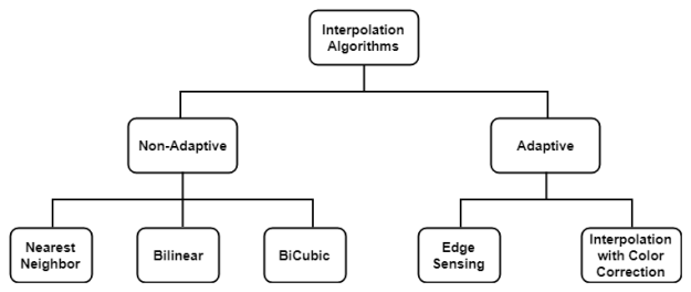
In the last blog, we discussed what is Bi-linear interpolation and how it is performed on images. In this blog, we will learn Bi-cubic interpolation in detail.

Note: We will be using some concepts from the Nearest Neighbour and Bilinear interpolation blog. Check them first before moving forward.

Difference between Bi-linear and Bi-cubic:

  1. Bi-linear uses 4 nearest neighbors to determine the output, while Bi-cubic uses 16 (4×4 neighbourhood).
  2. Weight distribution is done differently.

So, the only thing we need to know is how weights are distributed and rest is same as Bi-linear.

In OpenCV, weights are distributed according to the following code (whole code can be found here)

x used in the above code is calculated from below code where x = fx

Similarly, for y, replace x with fy and fy can be obtained by replacing dx and scale_x in the above code by dy and scale_y respectively (Explained in the previous blog).

Note: For Matlab, use A= -0.50

Let’s see an example. We take the same 2×2 image from the previous blog and want to upscale it by a factor of 2 as shown below

Steps:

  • In the last blog, we calculated for P1. This time let’s take ‘P2’. First, we find the position of P2 in the input image as we did before. So, we find P2 coordinate as (0.75,0.25) with dx = 1 and dy=0.
  • Because cubic needs 4 pixels (2 on left and 2 on right) so, we pad the input image.
  • OpenCV has different methods to add borders which you can check here. Here, I used cv2.BORDER_REPLICATE method. You can use any. After padding the input image looks like this
After padding, Blue square is the input image
  • To find the value of P2, let’s first visualize where P2 is in the image. Yellow is the input image before padding. We take the blue 4×4 neighborhood as shown below
  • For P2, using dx and dy we calculate fx and fy from code above. We get, fx=0.25 and fy=0.75
  • Now, we substitute fx and fy in the above code to calculate the four coefficients. Thus we get coefficients = [-0.0351, 0.2617,0.8789, -0.1055] for fy =0.75 and for fx=0.25 we get coefficients = [ -0.1055 , 0.8789, 0.2617, -0.0351]
  • First, we will perform cubic interpolation along rows( as shown in the above figure inside blue box) with the above calculated weights for fx as
    -0.1055 *10 + 0.8789*10 + 0.2617*20 -0.0351*20 = 12.265625
    -0.1055 *10 + 0.8789*10 + 0.2617*20 -0.0351*20 = 12.265625
    -0.1055 *10 + 0.8789*10 + 0.2617*20 -0.0351*20 = 12.265625
    -0.1055 *30 + 0.8789*30 + 0.2617*40 -0.0351*40 = 32.265625
  • Now, using above calculated 4 values, we will interpolate along columns using calculated weights for fy as
    -0.0351*12.265 + 0.2617*12.265 + 0.8789*12.265 -0.1055*32.625 = 10.11702
  • Similarly, repeat for other pixels.

The final result we get is shown below:

This produces noticeably sharper images than the previous two methods and balances processing time and output quality. That’s why it is used widely (e.g. Adobe Photoshop etc.)

In the next blog, we will see these interpolation methods using OpenCV functions on real images. Hope you enjoy reading.

If you have any doubt/suggestion please feel free to ask and I will do my best to help or improve myself. Good-bye until next time.

Changing Video Resolution using OpenCV-Python

In this tutorial, I will show how to change the resolution of the video using OpenCV-Python. This blog is based on interpolation methods (Chapter-5) which we have discussed earlier.

Here, I will convert a 640×480 video to 1280×720. Let’s see how to do this

Steps:

  1. Load a video using cv2.VideoCapture()
  2. Create a VideoWriter object using cv2.VideoWriter()
  3. Extract frame by frame
  4. Resize the frames using cv2.resize()
  5. Save the frames to a video file using cv2.VideoWriter()
  6. Release the VideoWriter and destroy all windows

Code:

Here, I have used Bicubic as the interpolation method, you can use any. Hope you enjoy reading.

If you have any doubt/suggestion please feel free to ask and I will do my best to help or improve myself. Good-bye until next time.

Image Interpolation using OpenCV-Python

In the previous blogs, we discussed the algorithm behind the

  1. nearest neighbor 
  2. bilinear and
  3. bicubic interpolation methods using a 2×2 image.

Now, let’s do the same using OpenCV on a real image. First, let’s take an image, either you can load one or can make own image. Loading an image from the device looks like this

This is a 20×22 apple image that looks like this.

Now, let’s zoom it 10 times using each interpolation method. The OpenCV command for doing this is

where fx and fy are scale factors along x and y, dsize refers to the output image size and the interpolation flag refers to which method we are going to use. Either you specify (fx, fy) or dsize, OpenCV calculates the other automatically. Let’s see how to use this function

Nearest Neighbor Interpolation

In this we use cv2.INTER_NEAREST as the interpolation flag in the cv2.resize() function as shown below

Output: 

Clearly, this produces a pixelated or blocky image. Also, it doesn’t introduce any new data.

Bilinear Interpolation

In this we use cv2.INTER_LINEAR flag as shown below

Output: 

This produces a smooth image than the nearest neighbor but the results for sharp transitions like edges are not ideal because the results are a weighted average of 2 surrounding pixels.

Bicubic Interpolation

In this we use cv2.INTER_CUBIC flag as shown below

Output: 

Clearly, this produces a sharper image than the above 2 methods. See the white patch on the left side of the apple. This method balances processing time and output quality fairly well.

Next time, when you are resizing an image using any software, wisely use the interpolation method as this can affect your result to a great extent. Hope you enjoy reading.

If you have any doubts/suggestions please feel free to ask and I will do my best to help or improve myself. Good-bye until next time.

Image Demosaicing or Interpolation methods

In the previous blog, we discussed the Bayer filter and how we can form a color image from a Bayer image. But we didn’t discuss much about interpolation or demosaicing algorithms so in this blog let’s discuss these algorithms in detail.

According to Wikipedia, Interpolation is a method of constructing new data points within the range of a discrete set of known data points. Image interpolation refers to the “guess” of intensity values at missing locations.

The big question is why we need interpolation if we are able to capture intensity values at all the pixels using Image sensor?

  1.  Bayer filter, where we need to find missing color information at each pixel.
  2.  Projecting low-resolution image to a high-resolution screen or vice versa. For example, we prefer watching videos in the full-screen mode.
  3.  Image Inpainting, Image Warping etc.
  4.  Geometric Transformations.

There are plenty of Interpolation methods available but we will discuss only the frequently used. Interpolation algorithms can be classified as

Non-adaptive perform interpolation in a fixed pattern for every pixel, while adaptive algorithms detect local spatial features, like edges, of the pixel neighborhood and make effective choices depending on the algorithm.

Let’s discuss the maths behind each interpolation method in the subsequent blogs.

In the next blog, we will see how the nearest neighbor method works. Hope you enjoy reading.

If you have any doubt/suggestion please feel free to ask and I will do my best to help or improve myself. Good-bye until next time.