Category Archives: Image Processing

Understanding Color Models using OpenCV-Python

In this blog, we will see how to convert images from one color model to another and how different colors can be obtained from these color models.

In OpenCV, the command for converting an image to another color-space is

cv2.cvtColor(input_image, conversion_method)

for example, BGR to HSV conversion can be done by using cv2.COLOR_BGR2HSV method

out_img = cv2.cvtColor(input_img, cv2.COLOR_BGR2HSV)

1	out_img = cv2.cvtColor(input_img, cv2.COLOR_BGR2HSV)

In OpenCV, more than 150 color-space conversion methods are available. To get the other conversion methods, type the following commands

>>> import cv2
>>> conver_method = [i for i in dir(cv2) if i.startswith('COLOR_')]
>>> print (conver_method)

>>> import cv2

>>> conver_method = [i for i in dir(cv2) if i.startswith('COLOR_')]

>>> print (conver_method)

In the previous blog, we learned how we can construct all colors from each model. Now, let’s get the feeling of this with OpenCV.

Here, I will create three trackbars to specify each of B, G, R colors and a window which shows the color obtained by combining different proportions of B, G, R. Similarly for HSI and CMYK models.

In OpenCV, Trackbar can be created using the cv2.createTrackbar() and its position at any moment can be found using cv2.getTrackbarPos().

RGB Trackbar

import cv2
import numpy as np

def nothing(x):
    pass

# Create a black image, a window
img = np.zeros((512,512,3), np.uint8)
cv2.namedWindow('image',cv2.WINDOW_NORMAl)

# create trackbars for color change
cv2.createTrackbar('R','image',0,255,nothing)
cv2.createTrackbar('G','image',0,255,nothing)
cv2.createTrackbar('B','image',0,255,nothing)


while True:
    cv2.imshow('image',img)
    if cv2.waitKey(1) & 0xFF == ord('q'):
        break
    
    # get current positions of three trackbars
    r = cv2.getTrackbarPos('R','image')
    g = cv2.getTrackbarPos('G','image')
    b = cv2.getTrackbarPos('B','image')

    img[:] = [b,g,r]

cv2.destroyAllWindows()

import cv2

import numpy as np

def nothing(x):

pass

# Create a black image, a window

img = np.zeros((512,512,3), np.uint8)

cv2.namedWindow('image',cv2.WINDOW_NORMAl)

# create trackbars for color change

cv2.createTrackbar('R','image',0,255,nothing)

cv2.createTrackbar('G','image',0,255,nothing)

cv2.createTrackbar('B','image',0,255,nothing)

while True:

cv2.imshow('image',img)

if cv2.waitKey(1) & 0xFF == ord('q'):

break

# get current positions of three trackbars

r = cv2.getTrackbarPos('R','image')

g = cv2.getTrackbarPos('G','image')

b = cv2.getTrackbarPos('B','image')

img[:] = [b,g,r]

cv2.destroyAllWindows()

You can move these trackbars to obtain different colors. A snapshot of output is shown below

HSI Trackbar

import cv2
import numpy as np

def nothing(x):
    pass

# Create a black image, a window
img = np.zeros((512,512,3), np.uint8)
cv2.namedWindow('image',cv2.WINDOW_NORMAL)

# create trackbars for color change
cv2.createTrackbar('H','image',0,180,nothing)
cv2.createTrackbar('S','image',0,255,nothing)
cv2.createTrackbar('I','image',0,255,nothing)

while(True):
    cv2.imshow('image',img)
    if cv2.waitKey(1) & 0xFF == ord('q'):
        break

    # get current positions of four trackbars
    r = cv2.getTrackbarPos('H','image')
    g = cv2.getTrackbarPos('S','image')
    b = cv2.getTrackbarPos('I','image')

    img[:,:] = [r,g,b]
    img = cv2.cvtColor(img, cv2.COLOR_HSV2BGR)

cv2.destroyAllWindows()

import cv2

import numpy as np

def nothing(x):

pass

# Create a black image, a window

img = np.zeros((512,512,3), np.uint8)

cv2.namedWindow('image',cv2.WINDOW_NORMAL)

# create trackbars for color change

cv2.createTrackbar('H','image',0,180,nothing)

cv2.createTrackbar('S','image',0,255,nothing)

cv2.createTrackbar('I','image',0,255,nothing)

while(True):

cv2.imshow('image',img)

if cv2.waitKey(1) & 0xFF == ord('q'):

break

# get current positions of four trackbars

r = cv2.getTrackbarPos('H','image')

g = cv2.getTrackbarPos('S','image')

b = cv2.getTrackbarPos('I','image')

img[:,:] = [r,g,b]

img = cv2.cvtColor(img, cv2.COLOR_HSV2BGR)

cv2.destroyAllWindows()

We get the following output as

Similarly, you can create trackbar for any color model. Play with these trackbars to get intuition about color models. Hope you enjoy reading.

If you have any doubt/suggestion please feel free to ask and I will do my best to help or improve myself. Good-bye until next time.

Object Tracking Using Color Models OpenCV-Python

Leave a reply

In this tutorial, we will learn how we can use color models for object tracking. You can use any color model. Here, I have used HSI because it is easier to represent a color using the HSI model (as it separates the color component from greyscale). Let’s see how to do this

Steps

Open the camera using cv2.VideoCapture()
Create 3 Trackbars of H, S, and I using cv2.createTrackbar()
Read frame by frame
Record the current trackbar position using cv2.getTrackbarPos()
Convert from BGR to HSV using cv2.cvtColor()
Threshold the HSV image based on current trackbar position using cv2.inRange()
Extract the desired result

Code

import cv2
import numpy as np

def nothing(x):
    pass

cap = cv2.VideoCapture(0) 

# Create a window
cv2.namedWindow('image',cv2.WINDOW_NORMAL)


# create trackbars for color change
cv2.createTrackbar('lowH','image',0,179,nothing)
cv2.createTrackbar('highH','image',179,179,nothing)

cv2.createTrackbar('lowS','image',0,255,nothing)
cv2.createTrackbar('highS','image',255,255,nothing)

cv2.createTrackbar('lowV','image',0,255,nothing)
cv2.createTrackbar('highV','image',255,255,nothing)

while(True):
    ret, frame = cap.read()

    # get current positions of the trackbars
    ilowH = cv2.getTrackbarPos('lowH', 'image')
    ihighH = cv2.getTrackbarPos('highH', 'image')
    ilowS = cv2.getTrackbarPos('lowS', 'image')
    ihighS = cv2.getTrackbarPos('highS', 'image')
    ilowV = cv2.getTrackbarPos('lowV', 'image')
    ihighV = cv2.getTrackbarPos('highV', 'image')

    hsv = cv2.cvtColor(frame, cv2.COLOR_BGR2HSV)
    lower_hsv = np.array([ilowH, ilowS, ilowV])
    higher_hsv = np.array([ihighH, ihighS, ihighV])
    mask = cv2.inRange(hsv, lower_hsv, higher_hsv)

    frame = cv2.bitwise_and(frame, frame, mask=mask)
    cv2.imshow('image', frame)
    if cv2.waitKey(1) & 0xFF == ord('q'):
        break

cap.release()
cv2.destroyAllWindows()

import cv2

import numpy as np

def nothing(x):

pass

cap = cv2.VideoCapture(0)

# Create a window

cv2.namedWindow('image',cv2.WINDOW_NORMAL)

# create trackbars for color change

cv2.createTrackbar('lowH','image',0,179,nothing)

cv2.createTrackbar('highH','image',179,179,nothing)

cv2.createTrackbar('lowS','image',0,255,nothing)

cv2.createTrackbar('highS','image',255,255,nothing)

cv2.createTrackbar('lowV','image',0,255,nothing)

cv2.createTrackbar('highV','image',255,255,nothing)

while(True):

ret, frame = cap.read()

# get current positions of the trackbars

ilowH = cv2.getTrackbarPos('lowH', 'image')

ihighH = cv2.getTrackbarPos('highH', 'image')

ilowS = cv2.getTrackbarPos('lowS', 'image')

ihighS = cv2.getTrackbarPos('highS', 'image')

ilowV = cv2.getTrackbarPos('lowV', 'image')

ihighV = cv2.getTrackbarPos('highV', 'image')

hsv = cv2.cvtColor(frame, cv2.COLOR_BGR2HSV)

lower_hsv = np.array([ilowH, ilowS, ilowV])

higher_hsv = np.array([ihighH, ihighS, ihighV])

mask = cv2.inRange(hsv, lower_hsv, higher_hsv)

frame = cv2.bitwise_and(frame, frame, mask=mask)

cv2.imshow('image', frame)

if cv2.waitKey(1) & 0xFF == ord('q'):

break

cap.release()

cv2.destroyAllWindows()

Open in full screen and play with trackbar to get more intuition about HSI model. Hope you enjoy reading.

If you have any doubt/suggestion please feel free to ask and I will do my best to help or improve myself. Good-bye until next time.

Color Models

Leave a reply

In the previous blogs, we represented the color image using the RGB components but this is not the only way available. There are different color models ( A color model is simply a way to define the color) available, each having their own pros and cons.

There are two types of color models available: Additive and Subtractive. Additive uses light (transmitted) to display color while subtractive models use printing inks. These models are fitted into different shapes to obtain new models (See HSI model below).

In this blog, we’ll discuss the three that are most commonly used in the context of digital image processing: RGB, CMY, and HSI

The RGB Color Model

In this, we construct a color cube whose 3 axes denote R, G, and B respectively as shown below

Normalized RGB Color Cube; Source: Researchgate

This is an additive model, i.e. the colors present in the light add to form new colors. For example, Yellow has coordinate of (1,1,0) which means Yellow = Red + Green. Similarly, for other colors like cyan = Blue + Green and magenta = Red +Blue.

R, G, and B are added together in varying proportions to produce an extensive range of colors. Mixing equal proportions of R, G, and B falls on the grayscale line.

Use: color monitors and most video cameras.

The CMYK Color Model

CMY stands for cyan, magenta, and yellow also known as secondary colors of light. K refers to black. An equal proportion of C, M, and Y produce muddly black and not pure black. That’s why we use CMYK instead of CMY model.

This is a subtractive model i.e colors are perceived as a result of reflected light. e.g. when light falls on a cyan coated surface, red is absorbed (or subtracted) while Green and Blue are reflected and thus G + B = Cyan. Similarly for magenta and yellow.

Thus, CMY can be obtained from RGB by subtracting RGB from the max intensity.

Use: Printing like books, magazines etc.

The HSI Color Model

HSI stands for Hue, Saturation, and Intensity. This model is similar to how humans perceive color. Let’s understand HSI terms

Hue: Color attribute that describes the pure color or dominant wavelength.

Saturation: Purity of Color or how much a pure color is diluted by white light.

Intensity: Amount of light

H and S tell us about the chromaticity (color information) of the light while I carries the greyscale information.

HSI model can be obtained by rotating the RGB cube such that Black is at the bottom and white at the top.

H varies from 0 to 120 degrees for Red, 120 – 240 for Green, and 240 -360 for Blue. Saturation can take value from 0 to 100%. Intensity value varies according to the bit size of an image.

Pros: Easier to represent the color than the RGB model.

Note: We can also use these color models for object tracking (See here).

In the next blog, we will see how different colors can be generated from these color models with the help of OpenCV. Hope you enjoy reading.

If you have any doubt/suggestion please feel free to ask and I will do my best to help or improve myself. Good-bye until next time.

Changing Video Resolution using OpenCV-Python

3 Replies

In this tutorial, I will show how to change the resolution of the video using OpenCV-Python. This blog is based on interpolation methods (Chapter-5) which we have discussed earlier.

Here, I will convert a 640×480 video to 1280×720. Let’s see how to do this

Steps:

Load a video using cv2.VideoCapture()
Create a VideoWriter object using cv2.VideoWriter()
Extract frame by frame
Resize the frames using cv2.resize()
Save the frames to a video file using cv2.VideoWriter()
Release the VideoWriter and destroy all windows

Code:

import cv2
import numpy as np

cap = cv2.VideoCapture('C:/New folder/video.avi')

fourcc = cv2.VideoWriter_fourcc(*'XVID')
out = cv2.VideoWriter('output.avi',fourcc, 5, (1280,720))

while True:
    ret, frame = cap.read()
    if ret == True:
        b = cv2.resize(frame,(1280,720),fx=0,fy=0, interpolation = cv2.INTER_CUBIC)
        out.write(b)
    else:
        break
    
cap.release()
out.release()
cv2.destroyAllWindows()

import cv2

import numpy as np

cap = cv2.VideoCapture('C:/New folder/video.avi')

fourcc = cv2.VideoWriter_fourcc(*'XVID')

out = cv2.VideoWriter('output.avi',fourcc, 5, (1280,720))

while True:

ret, frame = cap.read()

if ret == True:

b = cv2.resize(frame,(1280,720),fx=0,fy=0, interpolation = cv2.INTER_CUBIC)

out.write(b)

else:

break

cap.release()

out.release()

cv2.destroyAllWindows()

Here, I have used Bicubic as the interpolation method, you can use any. Hope you enjoy reading.

If you have any doubt/suggestion please feel free to ask and I will do my best to help or improve myself. Good-bye until next time.

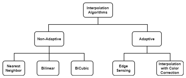
Image Interpolation using OpenCV-Python

Leave a reply

In the previous blogs, we discussed the algorithm behind the

nearest neighbor
bilinear and
bicubic interpolation methods using a 2×2 image.

Now, let’s do the same using OpenCV on a real image. First, let’s take an image, either you can load one or can make own image. Loading an image from the device looks like this

import cv2
import numpy as np

img = cv2.imread('C:/New folder/apple.jpg')

import cv2

import numpy as np

img = cv2.imread('C:/New folder/apple.jpg')

This is a 20×22 apple image that looks like this.

Now, let’s zoom it 10 times using each interpolation method. The OpenCV command for doing this is

dst = cv2.resize(src, dsize[, fx[, fy[, interpolation]]]])

1	dst = cv2.resize(src, dsize[, fx[, fy[, interpolation]]]])

where fx and fy are scale factors along x and y, dsize refers to the output image size and the interpolation flag refers to which method we are going to use. Either you specify (fx, fy) or dsize, OpenCV calculates the other automatically. Let’s see how to use this function

Nearest Neighbor Interpolation

In this we use cv2.INTER_NEAREST as the interpolation flag in the cv2.resize() function as shown below

near_img = cv2.resize(img,None, fx = 10, fy = 10, interpolation = cv2.INTER_NEAREST)

1	near_img = cv2.resize(img,None, fx = 10, fy = 10, interpolation = cv2.INTER_NEAREST)

Output:

Clearly, this produces a pixelated or blocky image. Also, it doesn’t introduce any new data.

Bilinear Interpolation

In this we use cv2.INTER_LINEAR flag as shown below

bilinear_img = cv2.resize(img,None, fx = 10, fy = 10, interpolation = cv2.INTER_LINEAR)

1	bilinear_img = cv2.resize(img,None, fx = 10, fy = 10, interpolation = cv2.INTER_LINEAR)

Output:

This produces a smooth image than the nearest neighbor but the results for sharp transitions like edges are not ideal because the results are a weighted average of 2 surrounding pixels.

Bicubic Interpolation

In this we use cv2.INTER_CUBIC flag as shown below

bicubic_img = cv2.resize(img,None, fx = 10, fy = 10, interpolation = cv2.INTER_CUBIC)

1	bicubic_img = cv2.resize(img,None, fx = 10, fy = 10, interpolation = cv2.INTER_CUBIC)

Output:

Clearly, this produces a sharper image than the above 2 methods. See the white patch on the left side of the apple. This method balances processing time and output quality fairly well.

Next time, when you are resizing an image using any software, wisely use the interpolation method as this can affect your result to a great extent. Hope you enjoy reading.

If you have any doubts/suggestions please feel free to ask and I will do my best to help or improve myself. Good-bye until next time.

Image Demosaicing or Interpolation methods

Leave a reply

In the previous blog, we discussed the Bayer filter and how we can form a color image from a Bayer image. But we didn’t discuss much about interpolation or demosaicing algorithms so in this blog let’s discuss these algorithms in detail.

According to Wikipedia, Interpolation is a method of constructing new data points within the range of a discrete set of known data points. Image interpolation refers to the “guess” of intensity values at missing locations.

The big question is why we need interpolation if we are able to capture intensity values at all the pixels using Image sensor?

Bayer filter, where we need to find missing color information at each pixel.
Projecting low-resolution image to a high-resolution screen or vice versa. For example, we prefer watching videos in the full-screen mode.
Image Inpainting, Image Warping etc.
Geometric Transformations.

There are plenty of Interpolation methods available but we will discuss only the frequently used. Interpolation algorithms can be classified as

Non-adaptive perform interpolation in a fixed pattern for every pixel, while adaptive algorithms detect local spatial features, like edges, of the pixel neighborhood and make effective choices depending on the algorithm.

Let’s discuss the maths behind each interpolation method in the subsequent blogs.

In the next blog, we will see how the nearest neighbor method works. Hope you enjoy reading.

If you have any doubt/suggestion please feel free to ask and I will do my best to help or improve myself. Good-bye until next time.

Bayer filter

Leave a reply

In the previous blog, we saw different methods by which color image can be obtained from an image sensor. Out of these methods, the Bayer filter is most widely used today and in this blog, we will discuss it in detail.

To form a color image, we need to collect information at RGB wavelengths for all the pixels or sensors. But this process is expensive both in terms of time and money.

So in 1976, Bayer thought of an alternative. Instead of capturing all RGB information at each pixel, Bayer thought of capturing one out of RGB for each pixel. Now, each pixel will contain either R, G or B. To be able to form a color image, he decided 50% pixels be Green and rest equally to Red and Blue (to mimic human eye) and these are arranged in a pattern as shown below

He would then use interpolation or color demosaicing algorithm to find the missing information for example pixel capturing Red will need Green and Blue and so on. We will study in more detail about interpolation algorithms in next blog.

The overall procedure from Bayer to RGB color image can be summarized as

Source: Thesis

So, with Bayer filter, we are only storing one color information(either R, G or B) at each pixel which reduces the computation time and cost while maintaining the image quality. That’s why it is used widely.

Hope you understand the Bayer filter, why it is used and how the color image is obtained from the Bayer image.Hope you enjoy reading.

If you have any doubt/suggestion please feel free to ask and I will do my best to help or improve myself. Good-bye until next time.

Understanding Images with OpenCV-Python

Leave a reply

In the previous blogs, we learned about pixels, intensity value, color, and greyscale image. Now, with OpenCV and numpy, let’s try to visualize these concepts.

First, we need an image, either you can load one or can make own image. Loading an image from the device looks like this

import cv2
import numpy as np

img = cv2.imread('F:/downloads/Python.png')

import cv2

import numpy as np

img = cv2.imread('F:/downloads/Python.png')

To access the pixel location, we must first know the shape of the image. This can be done by

>>> img.shape
(2000, 2000, 3)

1 2	>>> img.shape (2000, 2000, 3)

It returns a tuple of the number of rows, columns, and channels (if the image is color).

Total number of pixels can be found either by multiplying rows, columns, channels found using img.shape or by using the following command

>>> img.size          # same as 2000*2000*3
12000000

1 2	>>> img.size # same as 200020003 12000000

After knowing the image shape, we can access the pixel location by its row and column coordinates as

>>> img[250,250]                     # for single pixel
>>> img[280:340, 330:390]            # for image region

1 2	>>> img[250,250] # for single pixel >>> img[280:340, 330:390] # for image region

This returns the intensity value at that pixel location. For a greyscale image, intensity or pixel value is a single integer while for a color image, it is an array of Blue, Green, Red values.

# for color image, [Blue,Green,Red] value is returned
>>> img[250,250]
[157 166 200]
# for 8-bit greyscale image
>>> img[250,250]
257

# for color image, [Blue,Green,Red] value is returned

>>> img[250,250]

[157 166 200]

# for 8-bit greyscale image

>>> img[250,250]

257

Note: OpenCV reads the color image in BGR mode and not in RGB mode. Be careful

We know that intensity levels depend on the number of bits that can be found by

>>> img.dtype
dtype('uint8')           # 8-bit image

1 2	>>> img.dtype dtype('uint8') # 8-bit image

To access the RGB channels separately, use numpy indexing as shown below

>>> img[:,:,0]          # 0 for Blue, 1 - Green, 2 - Red

1	>>> img[:,:,0] # 0 for Blue, 1 - Green, 2 - Red

You can change the pixel value just by normal assignment as shown below

>>> img[250,250]
[0,0,0]
>>> img[250,250] = 34
>>> img[250,250]
[34,34,34]
# we can assign different values to each channel at a pixel
>>> img[250,250] = [234,145,23]
# to make all the red pixels to zero 
>>> img[:,:,2] = 0

>>> img[250,250]

[0,0,0]

>>> img[250,250] = 34

>>> img[250,250]

[34,34,34]

# we can assign different values to each channel at a pixel

>>> img[250,250] = [234,145,23]

# to make all the red pixels to zero

>>> img[:,:,2] = 0

You can change the color image to greyscale using the following command

grey = cv2.cvtColor(img, cv2.COLOR_BGR2GRAY)

1	grey = cv2.cvtColor(img, cv2.COLOR_BGR2GRAY)

All the operations that you can perform on the array like add, subtract etc apply to images also.

Play with all these commands to understand better. Hope you enjoy reading.

If you have any doubt/suggestion please feel free to ask and I will do my best to help or improve myself. Good-bye until next time.

Greyscale and Color Image

Leave a reply

In the previous blog, we learned how the digital image is formed but we didn’t discuss whether the image formed was greyscale or colored. In this blog, let’s go through this.

A greyscale image is the one where pixels contains only the intensity information and not wavelength. For example, a pixel value of 165 represents the amount of light captured by the sensor(pixel). It doesn’t tell how much of this light belongs to red wavelength or any other.

For an 8 bit image, there will be 2⁸=256 intensity levels where 0 means no light(black) and 255 means White light and in between levels represents shades of grey as shown below

The above image is created using numpy and OpenCV (See here for code).

A color image, on the other hand, contains intensity information corresponding to three wavelengths red, green, and blue (RGB)collectively called primary colors or channels. The reason for choosing these 3 colors lies in the fact that cone cells in the human eye, that is responsible for color vision, are sensitive to red, green, and blue light.

Note: Combining the primary colors(their wavelength may vary) in various intensity proportions, we can produce all visible colors.

So, in color image, corresponding to every pixel, we have 3 intensity values Red, Green, Blue (for example 160,30,45) that produces different colors in the image.

How a Color image is formed?

To form a color image, we want something that absorbs light in red, green, and blue wavelengths. The advancements in color image formation can be summarized by the figure below

Source: Foveon

The drastic advancement in color image formation came with the introduction of digital sensors like CCD and CMOS. Most of the digital cameras today only contain one imaging sensor so they cannot collect red, green, and blue information simultaneously at each pixel location. One possible solution is we use 3 imaging sensors with RGB filters but that is expensive in terms of money and time.

So, in 1976 Bryce Bayer of Eastman Kodak, invented the Bayer filter that revolutionized color image formation. Bayer filter is a color filter array(CFA) in which RGB color filters are arranged in a pattern on the sensor. Below figure shows a Bayer filter.

Source: Wikipedia

In the bayer filter, there are twice as many green elements as red or blue to mimic the human eye’s greater resolving power with the green light. In order to construct an RGB picture, we calculate Green and Blue values for each Red pixel, Blue and Red values for each Green pixel and Red and Green values for each Blue pixel through interpolation or color demosaicing algorithm (For more details See here).

Foveon X3 direct image sensor is the most advanced color image sensor. This combines the power of digital sensor with the essence of the film. Like the film, this has three layers of pixels embedded in silicon. The layers are positioned to take advantage of the fact that silicon absorbs red, green, and blue light to different depths. The bottom layer records red, the middle layer records green and the top layer records blue. Pros are superior quality and less processing power.

Now, you might have got some feeling about the Color image and how it is formed. Hope you enjoy reading.

If you have any doubt/suggestion please feel free to ask and I will do my best to help or improve myself. Good-bye until next time.

Create own image using Numpy and OpenCV

Leave a reply

In this tutorial, we will learn how we can create our own image using numpy and OpenCV. This will help you in understanding the image concepts more. Let’s see how the 256 intensity levels for an 8-bit image looks like.

Steps:

Create an array of any desired size using numpy. Always specify the ‘datatype’
Fill the values of the array using some logic
Show the image using cv2.imshow() or matplotlib.

Code:

import cv2
import numpy as np
import matplotlib.pyplot as plt

img = np.zeros((100,256),dtype=np.uint8)
for i in range(img.shape[1]):
    for j in range(img.shape[0]):
        img[j,i]=i

cv2.imshow('a',img)
cv2.waitKey(0)
cv2.destroyAllWindows()

#--------- using Matplotlib ------------
##plt.imshow(img, cmap = 'gray')
##plt.tick_params(axis='y',left = False,labelleft = False)
##plt.xticks([0,50,100,150,200,255])
##plt.show()

import cv2

import numpy as np

import matplotlib.pyplot as plt

img = np.zeros((100,256),dtype=np.uint8)

for i in range(img.shape[1]):

for j in range(img.shape[0]):

img[j,i]=i

cv2.imshow('a',img)

cv2.waitKey(0)

cv2.destroyAllWindows()

#--------- using Matplotlib ------------

##plt.imshow(img, cmap = 'gray')

##plt.tick_params(axis='y',left = False,labelleft = False)

##plt.xticks([0,50,100,150,200,255])

##plt.show()

The resulting image looks like this

To create a color image just specify the third dimension of the array (for example (100,256,3)) and rest is same.

Now, you are ready to create your own images. Hope you enjoy reading.

If you have any doubt/suggestion please feel free to ask and I will do my best to help or improve myself. Good-bye until next time.

TheAILearner

Mastering Artificial Intelligence

Category Archives: Image Processing

Understanding Color Models using OpenCV-Python

RGB Trackbar

HSI Trackbar

Object Tracking Using Color Models OpenCV-Python

Steps

Code

Color Models

The RGB Color Model

The CMYK Color Model

The HSI Color Model

Changing Video Resolution using OpenCV-Python

Steps:

Code:

Image Interpolation using OpenCV-Python

Nearest Neighbor Interpolation

Bilinear Interpolation

Bicubic Interpolation

Image Demosaicing or Interpolation methods

Bayer filter

Understanding Images with OpenCV-Python

Greyscale and Color Image

Create own image using Numpy and OpenCV

Steps:

Code: