In the previous blog, we learned how we can construct all colors from each model. Now, let’s get the feeling of this with OpenCV.
Here, I will create three trackbars to specify each of B, G, R colors and a window which shows the color obtained by combining different proportions of B, G, R. Similarly for HSI and CMYK models.
In OpenCV, Trackbar can be created using the cv2.createTrackbar() and its position at any moment can be found using cv2.getTrackbarPos().
RGB Trackbar
Python
1
2
3
4
5
6
7
8
9
10
11
12
13
14
15
16
17
18
19
20
21
22
23
24
25
26
27
28
29
importcv2
importnumpy asnp
defnothing(x):
pass
# Create a black image, a window
img=np.zeros((512,512,3),np.uint8)
cv2.namedWindow('image',cv2.WINDOW_NORMAl)
# create trackbars for color change
cv2.createTrackbar('R','image',0,255,nothing)
cv2.createTrackbar('G','image',0,255,nothing)
cv2.createTrackbar('B','image',0,255,nothing)
whileTrue:
cv2.imshow('image',img)
ifcv2.waitKey(1)&0xFF==ord('q'):
break
# get current positions of three trackbars
r=cv2.getTrackbarPos('R','image')
g=cv2.getTrackbarPos('G','image')
b=cv2.getTrackbarPos('B','image')
img[:]=[b,g,r]
cv2.destroyAllWindows()
You can move these trackbars to obtain different colors. A snapshot of output is shown below
HSI Trackbar
HSI Trackbar
Python
1
2
3
4
5
6
7
8
9
10
11
12
13
14
15
16
17
18
19
20
21
22
23
24
25
26
27
28
29
importcv2
importnumpy asnp
defnothing(x):
pass
# Create a black image, a window
img=np.zeros((512,512,3),np.uint8)
cv2.namedWindow('image',cv2.WINDOW_NORMAL)
# create trackbars for color change
cv2.createTrackbar('H','image',0,180,nothing)
cv2.createTrackbar('S','image',0,255,nothing)
cv2.createTrackbar('I','image',0,255,nothing)
while(True):
cv2.imshow('image',img)
ifcv2.waitKey(1)&0xFF==ord('q'):
break
# get current positions of four trackbars
r=cv2.getTrackbarPos('H','image')
g=cv2.getTrackbarPos('S','image')
b=cv2.getTrackbarPos('I','image')
img[:,:]=[r,g,b]
img=cv2.cvtColor(img,cv2.COLOR_HSV2BGR)
cv2.destroyAllWindows()
We get the following output as
Similarly, you can create trackbar for any color model. Play with these trackbars to get intuition about color models. Hope you enjoy reading.
If you have any doubt/suggestion please feel free to ask and I will do my best to help or improve myself. Good-bye until next time.
In this tutorial, we will learn how we can use color models for object tracking. You can use any color model. Here, I have used HSI because it is easier to represent a color using the HSI model (as it separates the color component from greyscale). Let’s see how to do this
Steps
Open the camera using cv2.VideoCapture()
Create 3 Trackbars of H, S, and I using cv2.createTrackbar()
Read frame by frame
Record the current trackbar position using cv2.getTrackbarPos()
Convert from BGR to HSV using cv2.cvtColor()
Threshold the HSV image based on current trackbar position using cv2.inRange()
In the previous blogs, we represented the color image using the RGB components but this is not the only way available. There are different color models ( A color model is simply a way to define the color) available, each having their own pros and cons.
There are two types of color models available: Additive and Subtractive. Additive uses light (transmitted) to display color while subtractive models use printing inks. These models are fitted into different shapes to obtain new models (See HSI model below).
In this blog, we’ll discuss the three that are most commonly used in the context of digital image processing: RGB, CMY, and HSI
The RGB Color Model
In this, we construct a color cube whose 3 axes denote R, G, and B respectively as shown below
This is an additive model, i.e. the colors present in the light add to form new colors. For example, Yellow has coordinate of (1,1,0) which means Yellow = Red + Green. Similarly, for other colors like cyan = Blue + Green and magenta = Red +Blue.
R, G, and B are added together in varying proportions to produce an extensive range of colors. Mixing equal proportions of R, G, and B falls on the grayscale line.
Use: color monitors and most video cameras.
The CMYK Color Model
CMY stands for cyan, magenta, and yellow also known as secondary colors of light. K refers to black. An equal proportion of C, M, and Y produce muddly black and not pure black. That’s why we use CMYK instead of CMY model.
This is a subtractive model i.e colors are perceived as a result of reflected light. e.g. when light falls on a cyan coated surface, red is absorbed (or subtracted) while Green and Blue are reflected and thus G + B = Cyan. Similarly for magenta and yellow.
Thus, CMY can be obtained from RGB by subtracting RGB from the max intensity.
Use: Printing like books, magazines etc.
The HSI Color Model
HSI stands for Hue, Saturation, and Intensity. This model is similar to how humans perceive color. Let’s understand HSI terms
Hue: Color attribute that describes the pure color or dominant wavelength.
Saturation: Purity of Color or how much a pure color is diluted by white light.
Intensity: Amount of light
H and S tell us about the chromaticity (color information) of the light while I carries the greyscale information.
HSI model can be obtained by rotating the RGB cube such that Black is at the bottom and white at the top.
H varies from 0 to 120 degrees for Red, 120 – 240 for Green, and 240 -360 for Blue. Saturation can take value from 0 to 100%. Intensity value varies according to the bit size of an image.
Pros: Easier to represent the color than the RGB model.
Note: We can also use these color models for object tracking (See here).
In the next blog, we will see how different colors can be generated from these color models with the help of OpenCV. Hope you enjoy reading.
If you have any doubt/suggestion please feel free to ask and I will do my best to help or improve myself. Good-bye until next time.
In this tutorial, I will show how to change the resolution of the video using OpenCV-Python. This blog is based on interpolation methods (Chapter-5) which we have discussed earlier.
Here, I will convert a 640×480 video to 1280×720. Let’s see how to do this
Steps:
Load a video using cv2.VideoCapture()
Create a VideoWriter object using cv2.VideoWriter()
Extract frame by frame
Resize the frames using cv2.resize()
Save the frames to a video file using cv2.VideoWriter()
Now, let’s do the same using OpenCV on a real image. First, let’s take an image, either you can load one or can make own image. Loading an image from the device looks like this
Python
1
2
3
4
importcv2
importnumpy asnp
img=cv2.imread('C:/New folder/apple.jpg')
This is a 20×22 apple image that looks like this.
Now, let’s zoom it 10 times using each interpolation method. The OpenCV command for doing this is
where fx and fy are scale factors along x and y, dsize refers to the output image size and the interpolation flag refers to which method we are going to use. Either you specify (fx, fy) or dsize, OpenCV calculates the other automatically. Let’s see how to use this function
Nearest Neighbor Interpolation
In this we use cv2.INTER_NEAREST as the interpolation flag in the cv2.resize() function as shown below
This produces a smooth image than the nearest neighbor but the results for sharp transitions like edges are not ideal because the results are a weighted average of 2 surrounding pixels.
Bicubic Interpolation
In this we use cv2.INTER_CUBIC flag as shown below
Clearly, this produces a sharper image than the above 2 methods. See the white patch on the left side of the apple. This method balances processing time and output quality fairly well.
Next time, when you are resizing an image using any software, wisely use the interpolation method as this can affect your result to a great extent. Hope you enjoy reading.
If you have any doubts/suggestions please feel free to ask and I will do my best to help or improve myself. Good-bye until next time.
In the previous blog, we discussed the Bayer filter and how we can form a color image from a Bayer image. But we didn’t discuss much about interpolation or demosaicing algorithms so in this blog let’s discuss these algorithms in detail.
According to Wikipedia, Interpolation is a method of constructing new data points within the range of a discrete set of known data points. Image interpolation refers to the “guess” of intensity values at missing locations.
The big question is why we need interpolation if we are able to capture intensity values at all the pixels using Image sensor?
Bayer filter, where we need to find missing color information at each pixel.
Projecting low-resolution image to a high-resolution screen or vice versa. For example, we prefer watching videos in the full-screen mode.
Image Inpainting, Image Warping etc.
Geometric Transformations.
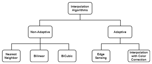
There are plenty of Interpolation methods available but we will discuss only the frequently used. Interpolation algorithms can be classified as
Non-adaptive perform interpolation in a fixed pattern for every pixel, while adaptive algorithms detect local spatial features, like edges, of the pixel neighborhood and make effective choices depending on the algorithm.
Let’s discuss the maths behind each interpolation method in the subsequent blogs.
In the next blog, we will see how the nearest neighbor method works. Hope you enjoy reading.
If you have any doubt/suggestion please feel free to ask and I will do my best to help or improve myself. Good-bye until next time.
Variational autoencoders are an extension of autoencoders and used as generative models. You can generate data like text, images and even music with the help of variational autoencoders.
Autoencoders are the neural network used to reconstruct original input. To know more about autoencoders please got through this blog. They have a certain application like denoising autoencoders and dimensionality reduction for data visualization. But apart from that, they are fairly limited.
To overcome this limitation, variational autoencoders comes into place. A common autoencoder learns a function which does not train autoencoder to generate images from a particular distribution. Also, if you try to create a generative model using autoencoders, you do not want to generate data as therein input. You want the output data with some variations which mostly look like input data.
Variational Autoencoder Model
A variational autoencoder has encoder and decoder part mostly same as autoencoders, the difference is instead of creating a compact distribution from its encoder, it learns a latent variable model. These latent variables are used to create a probability distribution from which input for the decoder is generated. Another is, instead of using mean squared or cross entropy loss function (as in autoencoders ) it has its own loss function.
I will not go further into the mathematics behind it, Lets jump into the code which will give more understanding about variational autoencoders. To know more about the mathematics behind it please go through this tutorial.
I have implemented variational autoencoder in keras using MNIST dataset. So lets first download the data.
Python
1
2
3
4
5
6
7
8
9
10
# download training and test data from mnist and reshape it
Now encode the output of the encoder to latent distribution parameters. Here, I have created two parameters mu and sigma which represents the mean and standard distribution of the distribution.
Here I have taken latent space dimension equal to 2. This is the bottleneck which means we are passing our entire set of data to two single variables. So if we increase our latent space dimension to 5, 10 or higher, we can get better results in the output. But this will create more data in the bottleneck.
Now create a Gaussian distribution function with mean zero and standard deviation of 1. This distribution will give variation in the input to the decoder, which will help to get variation in the output. Then decoder will predict the output using distribution.
Python
1
2
3
4
5
6
7
8
9
10
11
12
13
14
15
16
17
18
19
20
21
22
# create latent distribution function and generate vectors
For the loss function, a variational autoencoder uses the sum of two losses, one is the generative loss which is a binary cross entropy loss and measures how accurately the image is predicted, another is the latent loss, which is KL divergence loss, measures how closely a latent variable match Gaussian distribution. This KL divergence makes sure that our distribution generated from encoder do not go away from the origin. Then train the model.
Our model is ready and we can generate images from it very easily. All we need to do is sample latent variable from distribution and pass it to the decoder. Lets test with the following code:
Python
1
2
3
4
5
6
7
8
9
10
11
12
13
14
15
16
17
18
19
20
n=15# figure with 15x15 digits
digit_size=28
figure=np.zeros((digit_size*n,digit_size*n))
grid_x=np.linspace(-1,1,n)
grid_y=np.linspace(-1,1,n)
fori,yi inenumerate(grid_x):
forj,xi inenumerate(grid_y):
z_sample=np.array([[xi,yi]])*1.
x_decoded=decoder.predict(z_sample)
digit=x_decoded[0].reshape(digit_size,digit_size)
figure[i*digit_size:(i+1)*digit_size,
j*digit_size:(j+1)*digit_size]=digit
plt.figure(figsize=(10,10))
plt.imshow(figure)
plt.show()
Here is the output generated from sampled distribution in the above code.
In my previous blog, we have discussed what is an autoencoder, its applications and a simple implementation in keras. In this blog, we will see a variant of autoencoder – ‘ denoising autoencoders ‘.
A denoising autoencoder is an extension of autoencoders. An autoencoder tries to learn identity function( output equals to input ), which makes it risking to not learn useful feature. One method to overcome this problem is to use denoising autoencoders.
For training a denoising autoencoder, we need to use noisy input data. For that, we need to add some noise to an original image. The amount of corrupting data depends on the amount of information present in data. Usually, 25-30 % data is being corrupted. This can be higher if your data contains less information. Let see how you can add noise to data in code:
To calculate loss, the output of the denoising autoencoder is then compared to original input instead of the corrupted one. Such a loss function train model to learn interesting features rather than learning identity function.
I have implemented denoising autoencoder in keras using MNIST data, which will give you an overview, how a denoising autoencoder works.
Let’s start with a simple definition of autoencoders. ‘ Autoencoders are the neural networks trained to reconstruct their original input’.
Now, you might be thinking what’s the use of reconstructing same data. Let me give you an example If you want to transfer data of GB’s of size and somehow if you can compress it into MB’s and then able to reconstruct back the data to the original size, isn’t that a better way to transfer data. This is one of the applications of autoencoders.
Autoencoders generally consists of two parts, one is encoder and other is decoder. Encoder downscale data to less number of features and decoder upscale the extracted features to original one.
There are some practical applications of autoencoders:
Dimensionality reduction for data visualization
Image Denoising
Generative Models
Visualizing a 10-dimensional vector is difficult. To overcome this problem we need to reduce that 10-dimensional vector into 2-D or 3-D. One of the famous algorithm PCA (Principal Component Analysis) tries to solve this problem. PCA uses linear transformations while autoencoders can use both linear and non-linear transformations for dimensionality reduction. Which makes autoencoders to generate more complex and interesting features than PCA.
Autoencoders can be used to remove the noise present in the image. It can also be used to generate new images required for a specific task. We will see more about these two applications in the next blog.
Now, let’s start with the simple implementation of autoencoders in Keras using MNIST data. First, let’s download MNIST training and test data and reshape it.
MNIST data consists of images of digits. So, it is better to use a convolutional neural network in our encoders and decoders. In our encoder, I have used conv and max-pooling layers to extract the compressed representation. Then flatten the encoder output to 32 features. Which will be the input to the decoder.
In the decoder, we need to upsample the extracted 32 features into the original size of the image. To achieve this, I have used Conv2DTranspose functions from keras. Then the final layer of the decoder will give the reconstructed output which will be similar to the original input.
To minimize reconstruction loss, we train the network with a large dataset and update weights. Now, our model is created, the next thing is to compile and train the model.
Below are the results from autoencoder trained above. The first line of digits shows the original input (test images) while the second line represents the reconstructed inputs from the model.
Hope you understand the basics of autoencoders, where these can be used and how a simple autoencoder be implemented. In the next blog, we will see how to denoise an image using autoencoders. Hope you enjoy reading.
If you have any doubt/suggestion please feel free to ask and I will do my best to help or improve myself. Good-bye until next time.
Before moving forward, let’s first summarize what we have done till now. In the first blog, we created a snake game using pygame. Then in the next blog, using backpropagation, we let the neural network learn how to play snake game.
In this blog, we will let the genetic algorithm (GA) and neural network(NN) play the snake game (if you are new to genetic algorithm please refer to this blog).
But let’s first clear some doubts which are obvious to come in mind.
What is the advantage of using GA + NN?
We don’t need any training data.
Note: I am not saying this is better than backpropagation but for snake game problem creating a valid training data is a tough task so this is a good option other than reinforcement learning, which we will see later.
Where we will use GA in NN?
Instead of backpropagation, we will update weights using GA.
How we will use GA in NN?
This whole process can be easily summarized in 7 steps:
Creating a snake game and deciding neural network architecture.
Creating an initial population.
Deciding the fitness function.
Play a game for each individual in the population and sort each individual in the population based on the fitness function score.
Select a few top individuals from the population and create the remaining population from these top selected individuals using Crossover and mutation.
The new population is created (meaning the next generation).
Go to step 4 and repeat until the stopping criteria are not satisfied.
Now, I hope most of the things might be clear to you. Let’s see these steps in more detail
Creating a snake game and deciding neural network architecture
Snake game is created with pygame and network architecture is same as that of the previous blog with 7 units in the input layer, 3 units in the output layer with ‘softmax’ and used 2 hidden layers one of 9 units and other of 15 units with ‘relu’ as shown below.
Creating Initial Population
Here, I have chosen 50 individuals in the population and each individual is an array of weights of the neural network. Randomly initialize these individuals. See code below
1
2
3
4
5
6
7
8
9
10
11
12
13
# n_x no. of input units
# n_h no. of units in hidden layer 1
# n_h2 no. of units in hidden layer 2
# n_y no. of output units
# The population will have sol_per_pop chromosome where each chromosome has num_weights genes.
For each individual, a game is played and the fitness function is calculated which is then appended in the list as shown in the code below
1
2
3
4
5
6
7
8
9
def cal_pop_fitness(pop):
fitness=[]
foriinrange(pop.shape[0]):
fit=run_game_with_ML(display,clock,pop[i])
print('fitness value of chromosome '+str(i)+' : ',fit)
fitness.append(fit)
returnnp.array(fitness)
fitness=cal_pop_fitness(new_population)
Selection, Crossover, and Mutation (Step – 5)
Selection: Now, according to fitness value, some best individuals will be selected from the population and are stored in the ‘parents’ array as shown in the code below
1
2
3
4
5
6
7
8
9
10
11
def select_mating_pool(pop,fitness,num_parents):
# Selecting the best individuals in the current generation as parents for producing the offspring of the next generation.
Crossover: To produce children for the next generation, the crossover is used. First, two individuals are randomly selected from the best, then I randomly choose some values from first and some from the second individual to produce new offspring. This process is repeated until the total population size is not achieved as shown below
Mutation: Then, some variations are being added to the newly formed offspring. Here, for each child, I randomly selected 25 weights and mutated them by adding some random value as shown in the code below
With the help of fitness function, crossover and mutation, new population for the next generation is created. Now, next thing is to replace the previous population with this newly formed. Below is the code for this
1
2
3
# Creating the new population based on the parents and offspring.
Now we will repeat this process until our target for certain game score is not achieved. In this problem, I have used 100 generations for training and 2500 steps in a game, which was able to achieve a maximum score of 40. You can choose more number of steps per game and can achieve more score.


